• Prof. Brian L. Evans• Dept. of Electrical and Computer Engineering• The University of Texas at Austin

EE 345S Real-Time Digital Signal Processing Lab Spring 2006

Signals and Systems

3 - 2

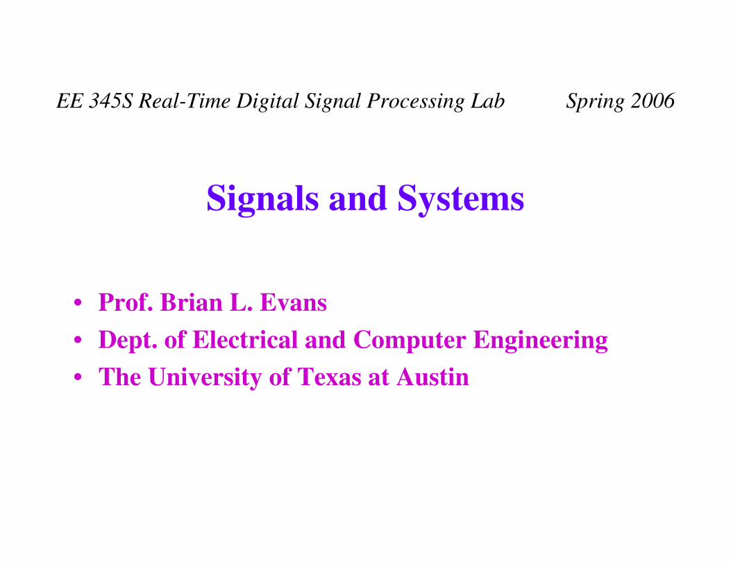
Signals As Functions of Time• Continuous-time signals are functions of a real

argumentx(t) where time, t, can take any real valuex(t) may be 0 for a given range of values of t

• Discrete-time signals are functions of an argument that takes values from a discrete setx[k] where k ∈ {...-3,-2,-1,0,1,2,3...}Integer time index, e.g. k, for discrete-time systems

• Values for x may be real or complex

Review

3 - 3

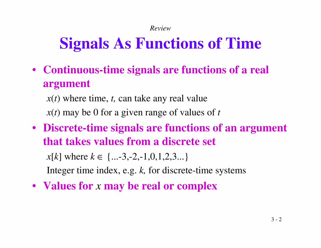
Analog vs. Digital Signals• Analog:

– Continuous in both time and amplitude

• Digital:– Discrete in both time and amplitude

Review

-3 -2 2 3 4-1 10

3 - 4

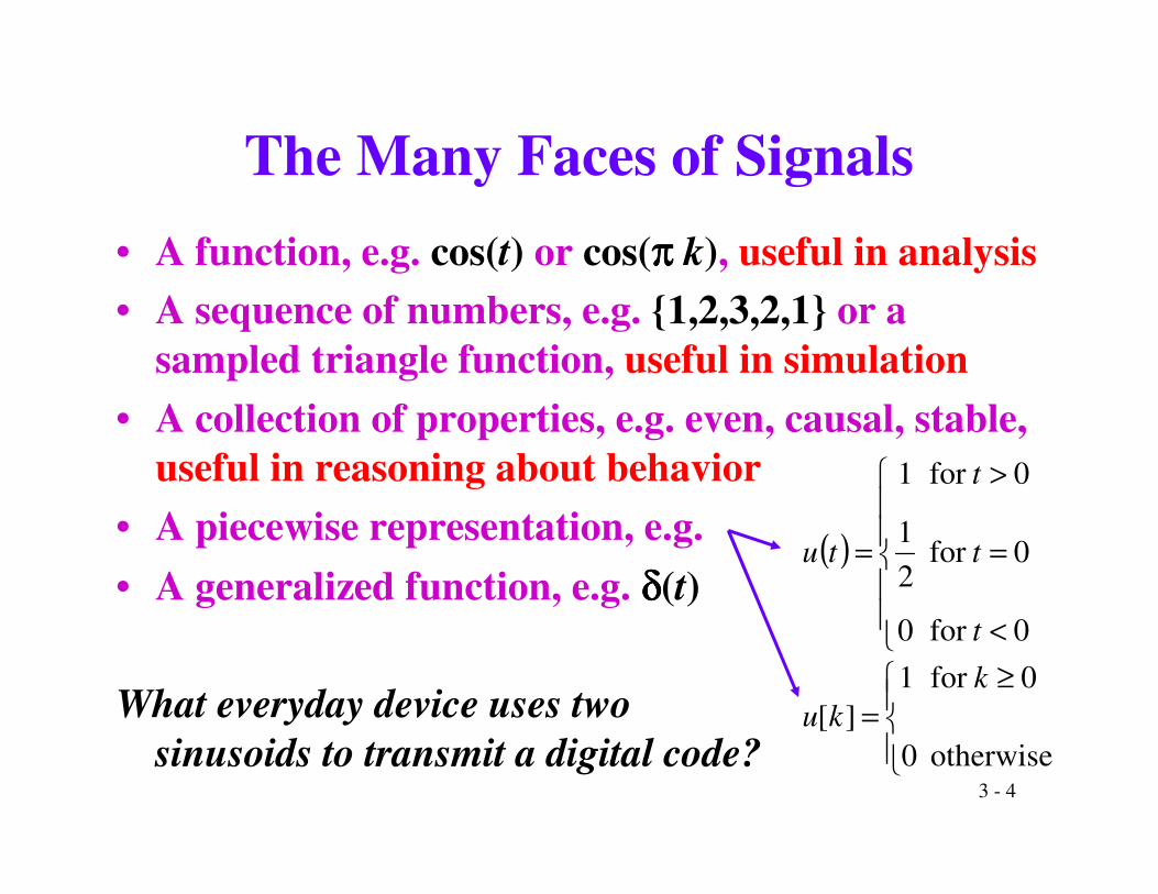
The Many Faces of Signals• A function, e.g. cos(t) or cos(ππππ k), useful in analysis• A sequence of numbers, e.g. {1,2,3,2,1} or a

sampled triangle function, useful in simulation• A collection of properties, e.g. even, causal, stable,

useful in reasoning about behavior• A piecewise representation, e.g.• A generalized function, e.g. δδδδ(t)

What everyday device uses twosinusoids to transmit a digital code?

( )

��

��

� ≥=

��

�

��

�

�

<

=

>

=

otherwise0

0for 1][

0for 0

0for 21

0for 1

kku

t

t

t

tu

3 - 5

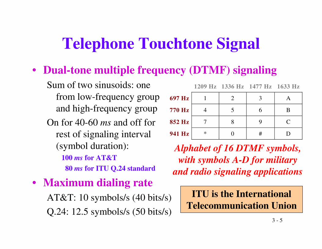
Telephone Touchtone Signal• Dual-tone multiple frequency (DTMF) signaling

Sum of two sinusoids: onefrom low-frequency groupand high-frequency group

On for 40-60 ms and off forrest of signaling interval(symbol duration):

100 ms for AT&T80 ms for ITU Q.24 standard

• Maximum dialing rateAT&T: 10 symbols/s (40 bits/s)Q.24: 12.5 symbols/s (50 bits/s)

1209 Hz 1336 Hz 1477 Hz 1633 Hz

697 Hz 1 2 3 A

770 Hz 4 5 6 B

852 Hz 7 8 9 C

941 Hz * 0 # D

Alphabet of 16 DTMF symbols, with symbols A-D for military

and radio signaling applications

ITU is the International Telecommunication Union

3 - 6

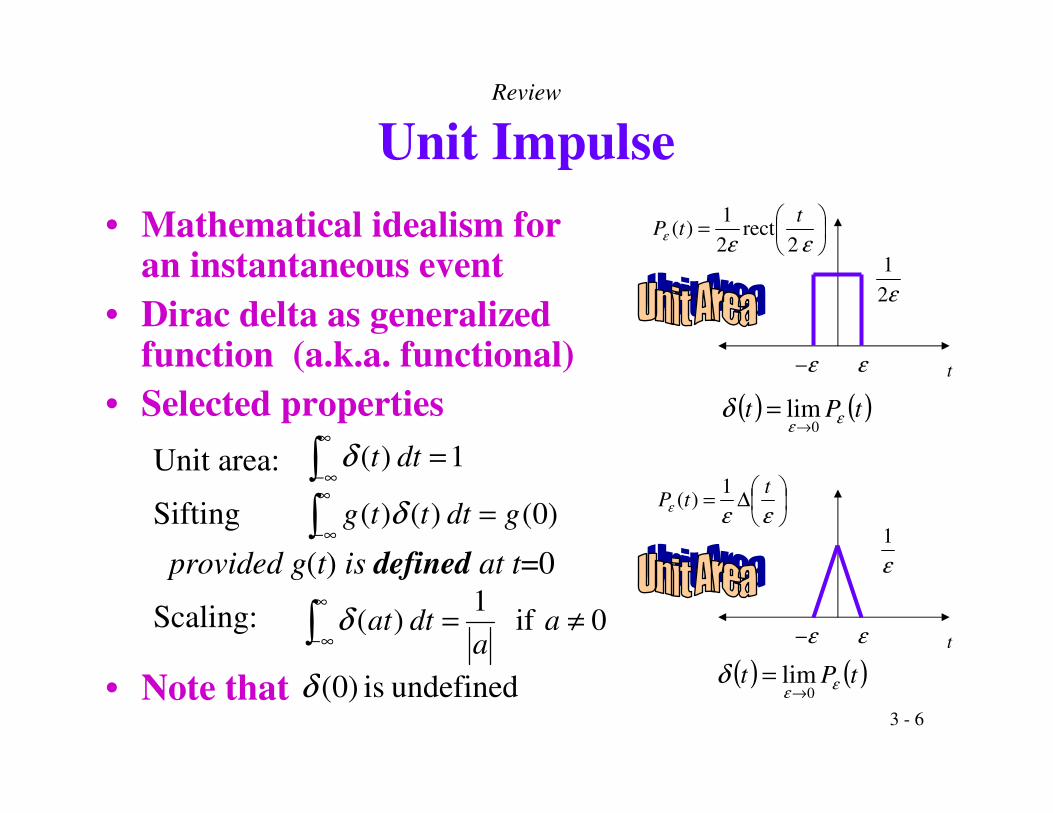
Unit Impulse• Mathematical idealism for

an instantaneous event• Dirac delta as generalized

function (a.k.a. functional)• Selected properties

Unit area:

Sifting

provided g(t) is defined at t=0

Scaling:

• Note that

�∞

∞−=1 )( dttδ

( ) ( )tPt εεδ

0lim

→=

ε−ε t

ε21

��

�

�=εεε 2

rect21

)(t

tP

Review

( ) ( )tPt εεδ

0lim

→=

ε−ε t

ε1

��

�

�∆=εεεt

tP1

)(�

∞

∞−= )0( )()( gdtttg δ

undefined is )0(δ

�∞

∞−≠= 0 if

1 )( a

adtatδ

3 - 7

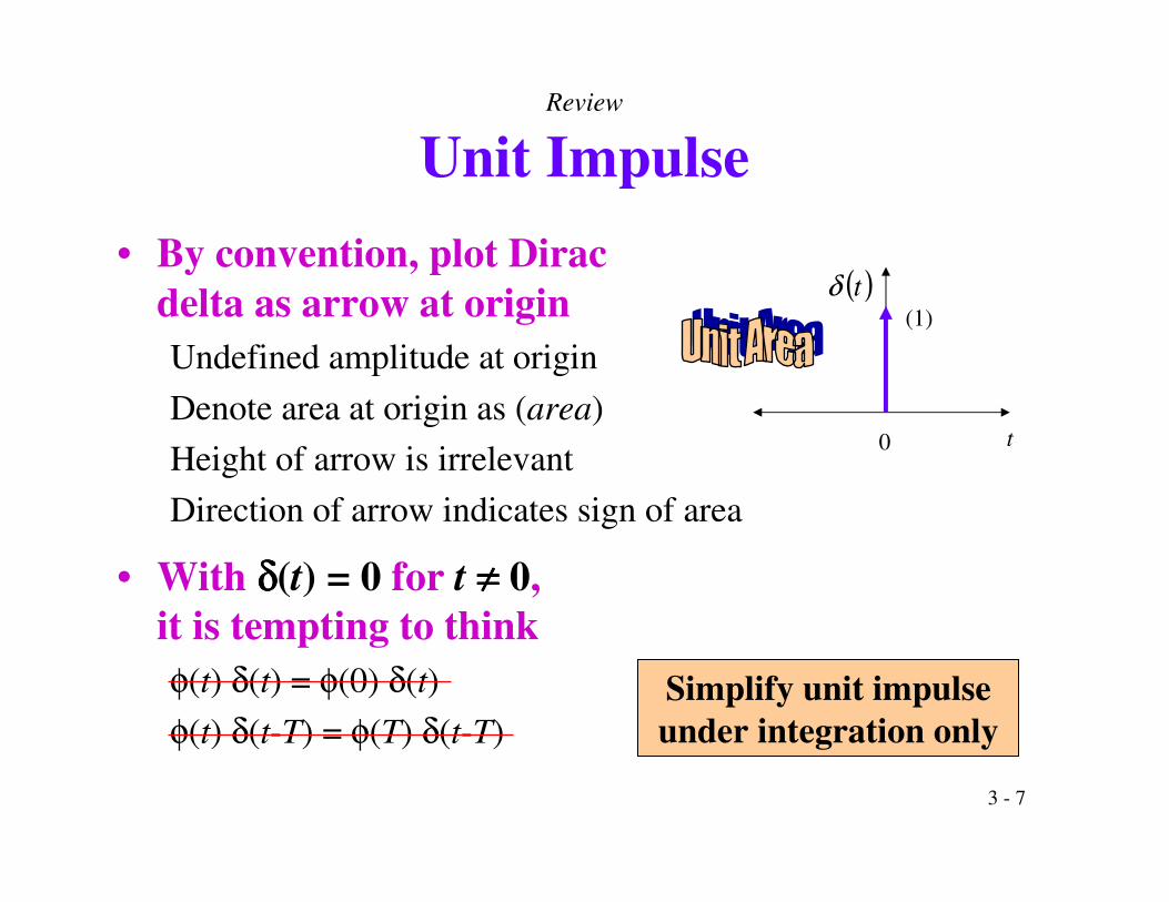
Unit Impulse• By convention, plot Dirac

delta as arrow at originUndefined amplitude at originDenote area at origin as (area)Height of arrow is irrelevantDirection of arrow indicates sign of area

• With δδδδ(t) = 0 for t ≠≠≠≠ 0,it is tempting to thinkφ(t) δ(t) = φ(0) δ(t)φ(t) δ(t-T) = φ(T) δ(t-T)

t

( )tδ(1)

0

Review

Simplify unit impulse under integration only

3 - 8

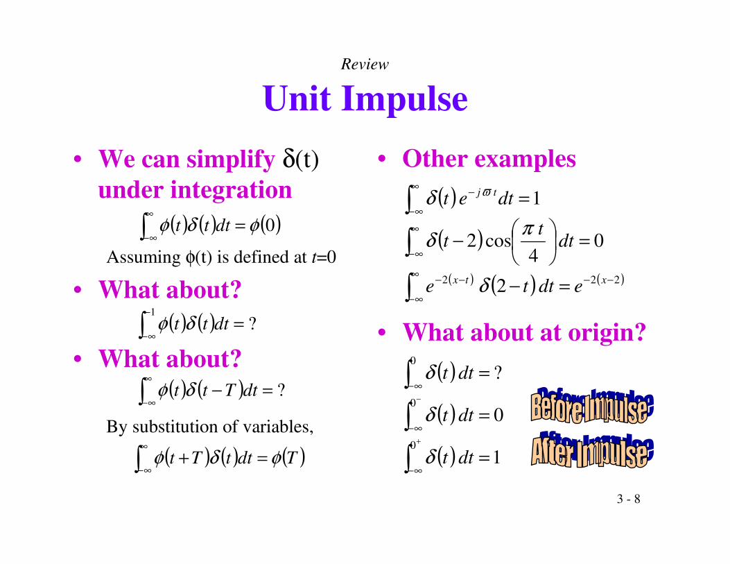
Unit Impulse• We can simplify δ(t)

under integration

Assuming φ(t) is defined at t=0

• What about?

• What about?

By substitution of variables,

• Other examples

• What about at origin?

( ) ( ) ( )�∞

∞−= 0φδφ dttt

( ) ( )�−

∞−=

1?dttt δφ

( ) ( )�∞

∞−=− ?dtTtt δφ

( ) ( ) ( )�∞

∞−=+ TdttTt φδφ

( )

( )( ) ( ) ( )

�

�

�

∞

∞−

−−−−

∞

∞−

∞

∞−

−

=−

=��

�

�−

=

222

2

0 4

cos 2

1

xtx

tj

edtte

dtt

t

dtet

δ

πδ

δ ϖ

( )

( )

( )�

�

�

+

−

∞−

∞−

∞−

=

=

=

0

0

0

1

0

?

dtt

dtt

dtt

δ

δ

δ

Review

3 - 9

( )tdtdu δ=( )

( )tu

tt

td

t

=

��

��

�

>=<

=� ∞−0100

?0

ττδ

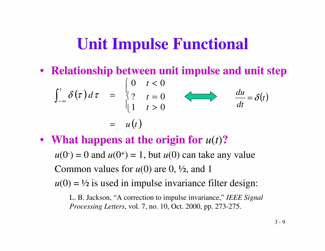
Unit Impulse Functional• Relationship between unit impulse and unit step

• What happens at the origin for u(t)?u(0-) = 0 and u(0+) = 1, but u(0) can take any valueCommon values for u(0) are 0, ½, and 1u(0) = ½ is used in impulse invariance filter design:

L. B. Jackson, “A correction to impulse invariance,” IEEE Signal Processing Letters, vol. 7, no. 10, Oct. 2000, pp. 273-275.

3 - 10

Systems• Systems operate on signals to produce new signals

or new signal representations

• Continuous-time examplesy(t) = ½ x(t) + ½ x(t-1)y(t) = x2(t)

• Discrete-time system examplesy[n] = ½ x[n] + ½ x[n-1]y[n] = x2[n]

Review

Squaring function can be used in sinusoidal demodulation

Average of current input and delayed input is a simple filter

( ) ( ){ } txTty = { } ][ ][ kxTky =

T{•} y(t)x(t) T{•} y[k]x[k]

3 - 11

System Properties• Let x(t), x1(t), and x2(t) be inputs to a continuous-

time linear system and let y(t), y1(t), and y2(t) be their corresponding outputs

• A linear system satisfiesAdditivity: x1(t) + x2(t) � y1(t) + y2(t)Homogeneity: a x(t) � a y(t) for any real/complex constant a

• For a time-invariant system, a shift of input signal by any real-valued τ causes same shift in output signal, i.e. x(t - τ) � y(t - τ) for all τ

Review

3 - 12

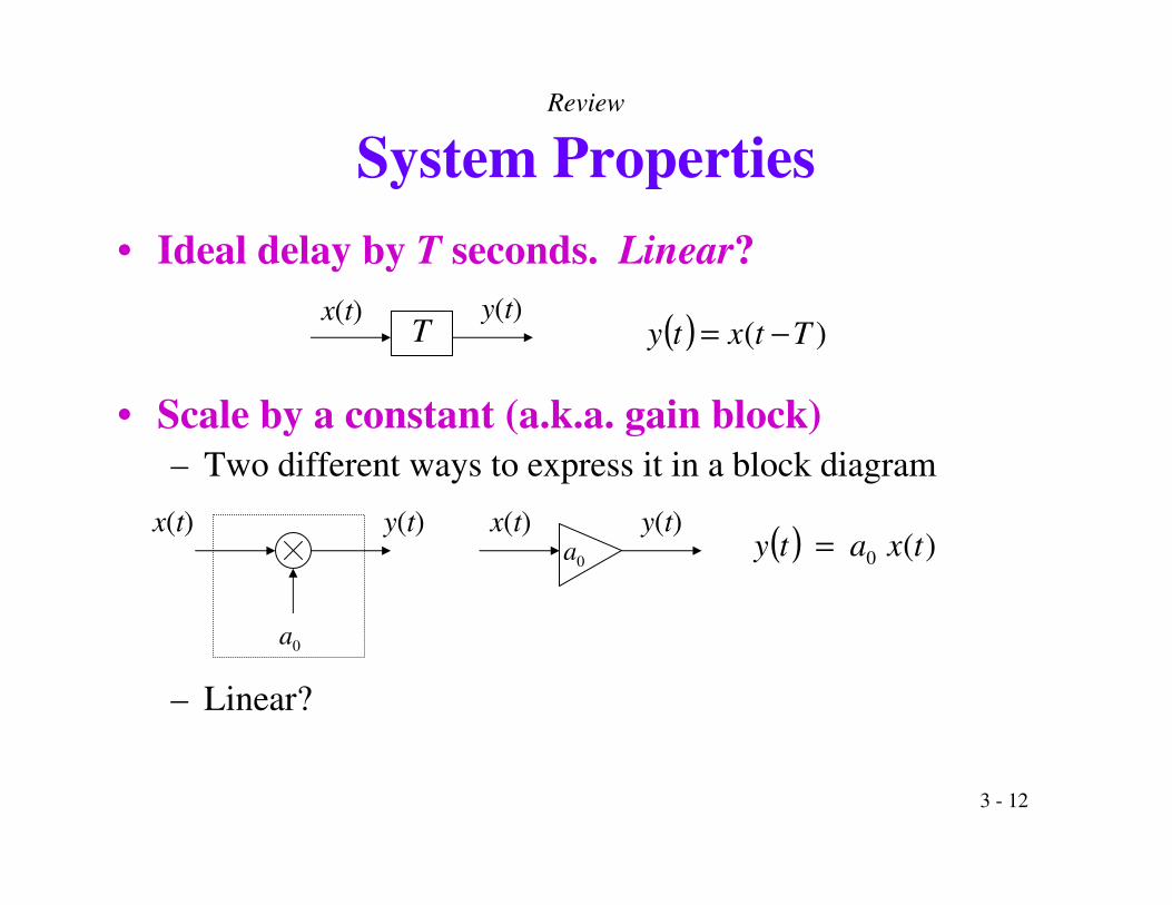
( ) )( Ttxty −=

System Properties• Ideal delay by T seconds. Linear?

• Scale by a constant (a.k.a. gain block)– Two different ways to express it in a block diagram

– Linear?

Tx(t) y(t)

0ax(t) y(t) ( ) )( 0 txaty =

0a

x(t) y(t)

Review

3 - 13

( ) ( ) −

=

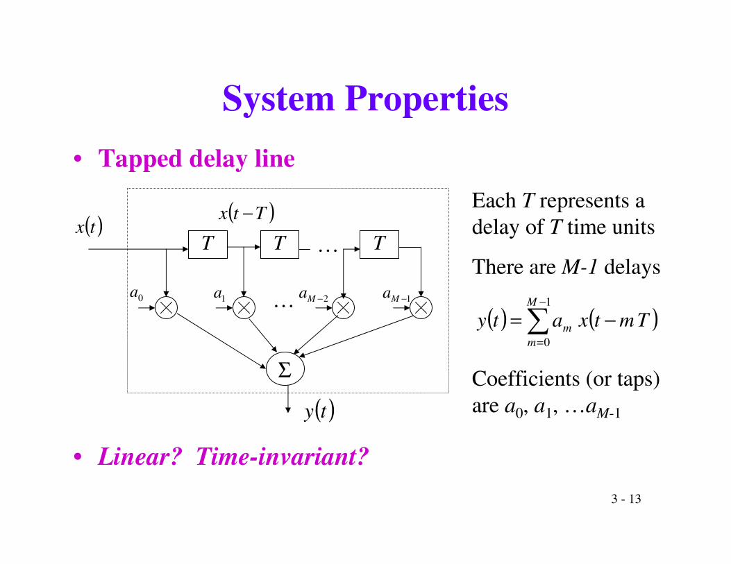
−=1

0

M

mm Tmtxaty

Each T represents a delay of T time units

System Properties• Tapped delay line

• Linear? Time-invariant?

There are M-1 delays

( )txT TT

Σ

( )ty

0a 1−Ma2−Ma1a …

…( )Ttx −

Coefficients (or taps) are a0, a1, …aM-1

3 - 14

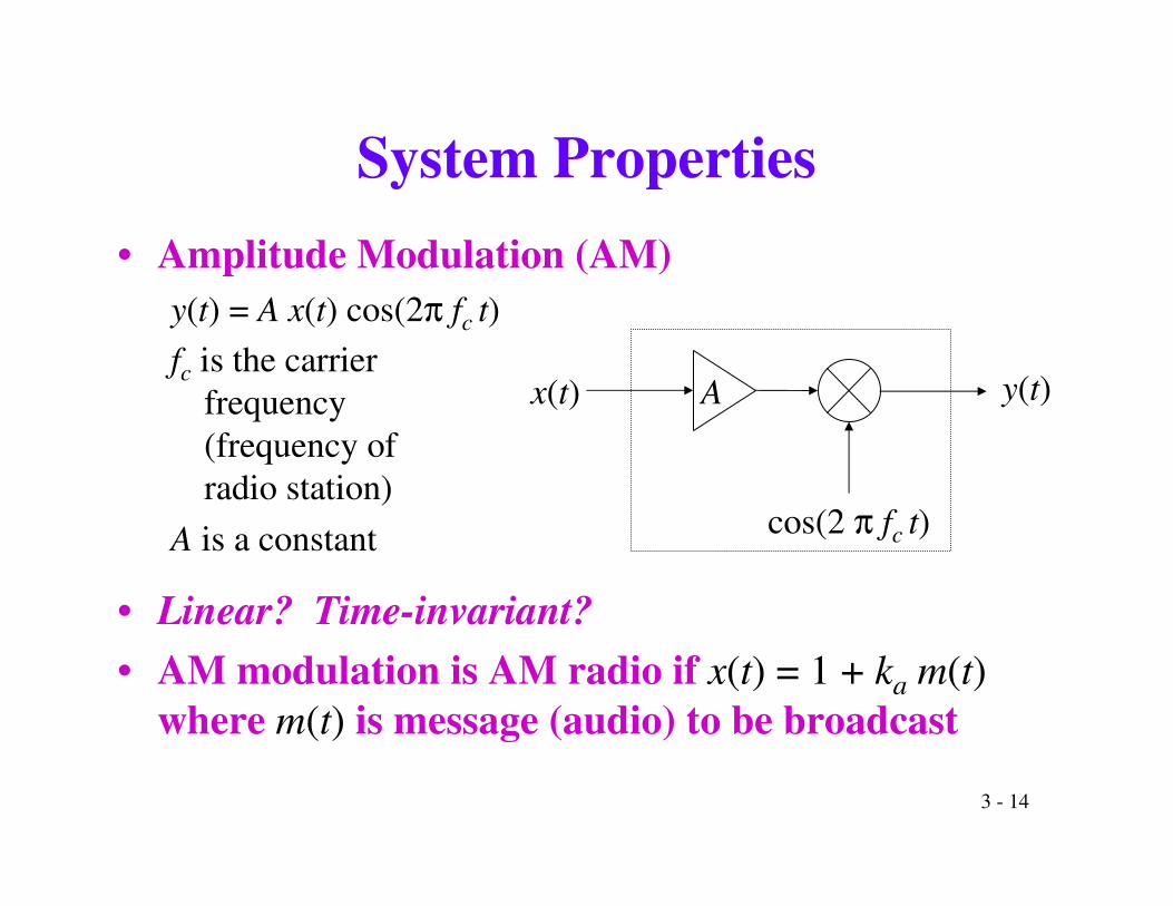
System Properties• Amplitude Modulation (AM)

y(t) = A x(t) cos(2π fc t)fc is the carrier

frequency(frequency ofradio station)

A is a constant

• Linear? Time-invariant?• AM modulation is AM radio if x(t) = 1 + ka m(t)

where m(t) is message (audio) to be broadcast

Ax(t)

cos(2 π fc t)

y(t)

3 - 15

( ) ( ) ���

�

�+= �

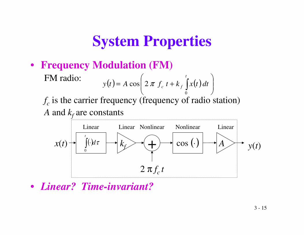
t

fc dttxktfAty0

2cos π

System Properties• Frequency Modulation (FM)

FM radio:

fc is the carrier frequency (frequency of radio station)A and kf are constants

• Linear? Time-invariant?

+kfx(t) A

2 π fc t

Linear Linear Nonlinear Nonlinear Linear

( ) τdt

� ⋅0

( )⋅cos y(t)

3 - 16

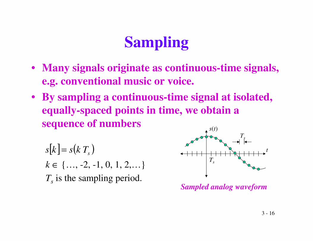
[ ] ( )sTksks =

Sampling• Many signals originate as continuous-time signals,

e.g. conventional music or voice.• By sampling a continuous-time signal at isolated,

equally-spaced points in time, we obtain a sequence of numbers

k ∈ {…, -2, -1, 0, 1, 2,…}Ts is the sampling period.

Sampled analog waveform

s(t)

t

Ts

Ts

3 - 17

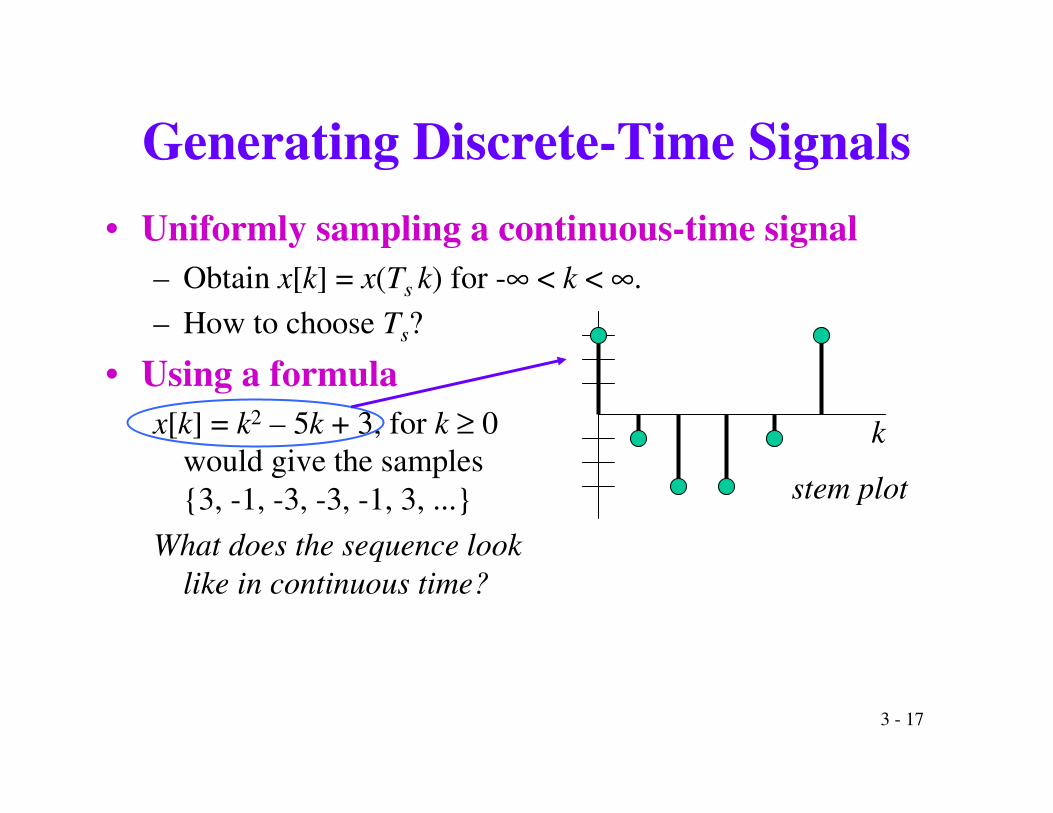
Generating Discrete-Time Signals• Uniformly sampling a continuous-time signal

– Obtain x[k] = x(Ts k) for -∞ < k < ∞.– How to choose Ts?

• Using a formulax[k] = k2 – 5k + 3, for k ≥ 0

would give the samples{3, -1, -3, -3, -1, 3, ...}

What does the sequence looklike in continuous time?

k

stem plot

3 - 18

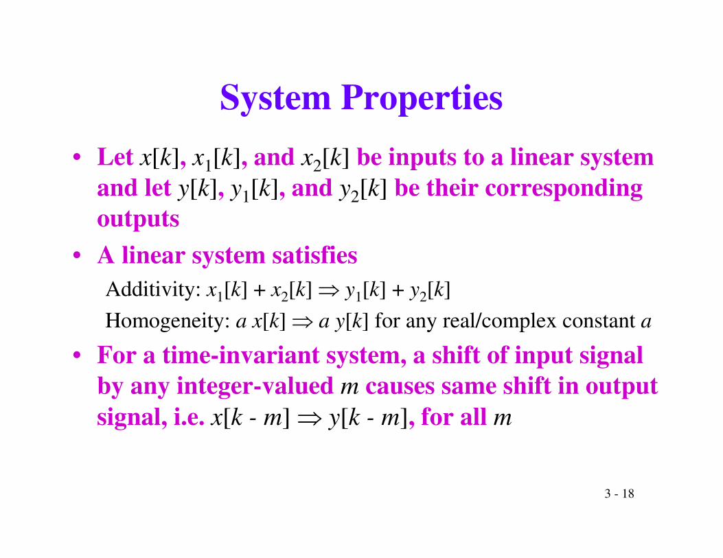
System Properties• Let x[k], x1[k], and x2[k] be inputs to a linear system

and let y[k], y1[k], and y2[k] be their corresponding outputs

• A linear system satisfiesAdditivity: x1[k] + x2[k] � y1[k] + y2[k]Homogeneity: a x[k] � a y[k] for any real/complex constant a

• For a time-invariant system, a shift of input signal by any integer-valued m causes same shift in output signal, i.e. x[k - m] � y[k - m], for all m

3 - 19

−

=

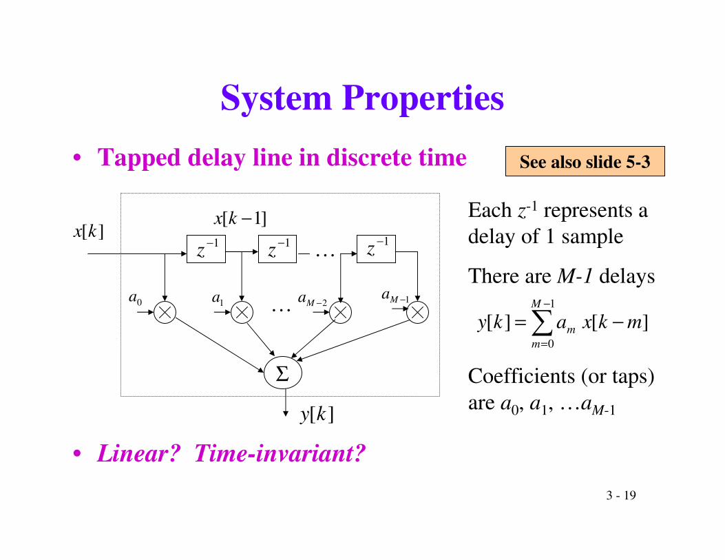
−=1

0

][ ][M

mm mkxaky

Each z-1 represents a delay of 1 sample

System Properties• Tapped delay line in discrete time

• Linear? Time-invariant?

There are M-1 delays

][kx1−z

Σ

][ky

0a 1−Ma2−Ma1a …

… 1−z1−z

]1[ −kx

See also slide 5-3

Coefficients (or taps) are a0, a1, …aM-1

3 - 20

System Properties• Continuous time

• Linear?• Time-invariant?

• Discrete time

• Linear?• Time-invariant?

( )⋅dtdf(t) y(t)

( ) ( ){ }( ) ( )

tttftf

tfdtd

ty

t ∆∆−−=

=

→∆ 0lim

[ ] ( ) ( ){ }( ) ( )

[ ] [ ]1

lim0

−−=

−−=

==

→

=

kfkf

TTkTfkTf

tfdtd

kTyky

s

sss

T

kTts

s

s

( )⋅dtd̂f[k] y[k]

See also slide 5-13

3 - 21

Conclusion• Continuous-time versus discrete-time:

discrete means quantized in timediscrete means quantized in time• Analog versus digital:

digital means quantized in time and amplitudedigital means quantized in time and amplitude• A digital signal processor (DSP) is a discrete-time

and digital systemA DSP processor is well-suited for implementing LTI digital

filters, as you will see in laboratory #3.

3 - 22

Signal Processing Systems• Speech synthesis and recognition• Audio CD players• Audio compression: MPEG 1 layer 3

audio (MP3), AC3• Image compression: JPEG, JPEG 2000• Optical character recognition• Video CDs: MPEG 1• DVD, digital cable, HDTV: MPEG 2• Wireless video: MPEG 4 Baseline/H.263,

MPEG 4 Adv. Video Coding/H.264 (emerging)• Examples of communication systems?

Moving Picture Experts Group

(MPEG)

Joint Picture Experts Group

(JPEG)

Optional

3 - 23

Communication Systems• Voiceband modems (56k)• Digital subscriber line (DSL) modems

ISDN: 144 kilobits per second (kbps)Business/symmetric: HDSL and HDSL2Home/asymmetric: ADSL, ADSL2, VDSL, and VDSL2

• Cable modems• Cellular phones

First generation (1G): AMPSSecond generation (2G): GSM, IS-95 (CDMA)Third generation (3G): cdma2000, WCDMA

Optional