Workshop Uncertainty Analysis in Geophysical Inverse Problems

Lorentz Center, Leiden, The Netherlands

A Few Concluding Comments …

Olivier TalagrandLaboratoire de Météorologie Dynamique, École Normale Supérieure, Paris, France

With Acknowledgments to M. Jardak, A. Fichtner, J. Trampert, P. J. van Leeuwenand all participants in the Workshop

11 November 2011

Vocabulary (e. g. ‘model’) !

- Summary and comments

- Ensemble estimation (resampling methods, Monte-Carlo or otherwise)

- A few problems to be solved

Bayesian vs. frequentist point of view (L. Tenorio, M. Holschneider, J. Trampert) ?

Bayesian estimation

The problem, if there is any, is with the prior.

But is there always a prior ?

First time geophysicists attempted to determine a ‘model’ of the Earth’s interior from observations of the propagation of seismic waves, did they have a prior ?

Early 2005. Huygens probe descended into the atmosphere of Titan (satellite of Saturn). No prior was used.

And, if there a prior, where does it come from, if not from earlier data ? L. Tenorio, who works on cosmological problems, mentioned he had a prior for the Universe, based on quantum fluctuations.

Bayesian estimation (continued)

Prior can be implicit

State vector x, belonging to state space S (dimS = n), to be estimated.

Data vector z, belonging to data space D (dimD = m), available.

z = F(x, ) (1)

where is a random element representing the uncertainty on the data (or, more precisely, on the link between the data and the unknown state vector).

For example

z = x +

Bayesian estimation (continued)

Probability that x = for given ?

x = z = F(, )

P(x = | z) = P[z = F(, )] / ’ P[z = F(’, )]

Unambiguously defined iff, for any , there is at most one x such that (1) is verified.

data contain information, either directly or indirectly, on any component of x. Determinacy condition.

No need for explicit knowledge for a prior probability distribution for x, but need for for explicit knowledge for probability distribution for .

Presentation by H. Igel (starting point m0 not associated with probability distribution)

ExampleExample

z = x + N [, S]

Then conditional probability distribution is

P(x z) = N [xa, Pa]where

xa = ( T S-1)-1 T S-1 [z] Pa = ( T S-1)-1

Determinacy condition : rank= n. Requires m ≥ n.

Expressions

xa = ( T S-1)-1 T S-1 [z] (2a) Pa = ( T S-1)-1 (2b)

can also be obtained, from the knowledge of only and S, as defining the variance minimizing linear estimator of x from z, or Best Linear Unbiased Estimate (BLUE) of x from z (but significance of Pa is now totally different)

Expressions (2) are commonly used, and are useful, in many (especially, but non only, geophysical) applications where error is distinctly non-gaussian and operator is mildly nonlinear. In fact, going beyond (2) turns out to be very challenging in many practical problems.

This Workshop

In addition to mathematical and theoretical papers, large variety of different physical applications and methods.

Beyond differences in vocabulary and notations, methods used are fundamentally the same. Linear and gaussian inversion (ray-tracing inversion, …) , heuristically extended to (mildly) nonlinear and non-gaussian situations, and sampling, or ‘ensemble’ methods, intended at explicitly sampling the uncertainty.

Seismic Tomography

Major development. Full Waveform Inversion. Is physics simpler for seismologists than for fluid dynamicists ?

Major problem of underdeterminacy. Null space matters, hence Backus-Gilbert theory (D. Al-Attar)

Sampling algorithms: Gibbs, Metropolis-Hastings, Neighbourhood Algorithm (M. Sambridge).

Neural network (NN, J. Trampert). Very efficient for numerical inversion of nonlinear functions. But link with bayesian approach and uncertainty quantification ?

Assimilation

The word assimilation refers to the situation when the observed system evolves in time and the dynamical laws which govern the evolution of the system are among the information to be used.

This does not change anything to the conceptual nature of the problem, but it means that in the description

z = F(x, )

the dynamical laws are present in a way or another.

Because they exist for producing daily forecasts, meteorologists started assimilation very early (A. Lorenc)

© Crown copyright Met Office Andrew Lorenc 14

ratio of supercomputer costs: 1 day's assimilation / 1 day forecast

5

8

20

31

1

10

100

1985 1990 1995 2000 2005 2010

AC scheme

3D-Var on T3E

simple 4D-Var on SX8

4D-Var with

outer_loop

Ratio of global computer costs: 1 day’s DA (total incl. FC) / 1 day’s forecast.

Computer power increased by 1M in 30 years.

Only 0.04% of the Moore’s Law increase over this time went into improved DA algorithms, rather than improved resolution!

Three classes of algorithms have been presented, with both specific applications and theoretical discussions

- Variational assimilation, which is a standard tool in meteorology, and has extended in recent years to applications in solid earth geophysics.

- Kalman filter, which is equivalent to variational assimilation in the linear case, and has been presented in its nonlinear extension, the Ensemble Kalman filter (EnKF)

- Particle filters, which are totally bayesian in their principle (P. J. van Leeuwen).

Assimilation, as it has done over the years, is continuously extending to more and more novel physical applications : geomagnetism (A. Fournier, A. Jackson), observations of the Earh’s rotation (J. Saynisch), atmospheric chemistry (H. Eskes), identification of CO2 surface fluxes (V. Gaur).

Theory : R. Potthast, P. J. Van Leeuwen

Very active field, which we can expect to further develop in the coming years, both through the development of new physical applications, and of theoretical methods.

Purely bayesian methods, particle filters ?

Quantification of uncertainty : identification and quantification of model (I mean ‘theory’) errors, and ensemble methods.

- Ensemble estimation (resampling methods, Monte-Carlo or otherwise)

ECMWF, Technical Report 499, 2006

Data

z = x +

Then conditional posterior probability distribution

P(x z) = N [xa, Pa]with

xa = ( T S-1)-1 T S-1 [z]Pa = ( T S-1)-1

Ready recipe for producing sample of independent realizations of posterior probability distribution (resampling method)

Perturb data vector additively according to error probability distribution N [0, S], and compute analysis xa for each perturbed data vector

Available data consist of

- Background estimate at time 0

x0b = x0

+ 0b 0

b N [, P0b]

- Observations at times k = 0, …, K

yk = Hkxk + k k N [, Rk]

- Model (supposed to be exact)

xk+1 = Mkxk k = 0, …, K-1

Errors assumed to be unbiased and uncorrelated in time, Hk and Mk linear

Then optimal state (mean of bayesian gaussian pdf) at initial time 0 minimizes objective function

0SJ(0) = (1/2) (x0

b - 0)T [P0b]-1 (x0

b - 0) + (1/2) k[yk - Hkk]T Rk-1 [yk - Hkk]

subject to k+1 = Mkk , k = 0, …, K-1

Work done here (with M. Jardak). Apply ‘ensemble’ recipe described above to nonlinear and non-gaussian cases, and look at what happens.

Everything synthetic, Two one-dimensional toy models : Lorenz ’96 model and Kuramoto-Sivashinsky equation. Perfect model assumption

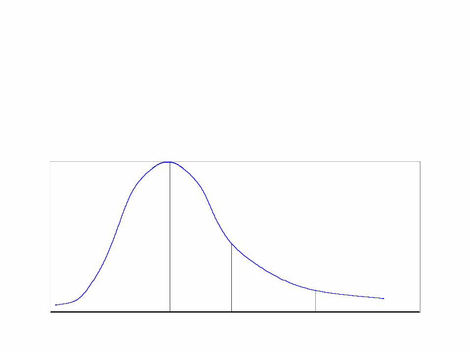
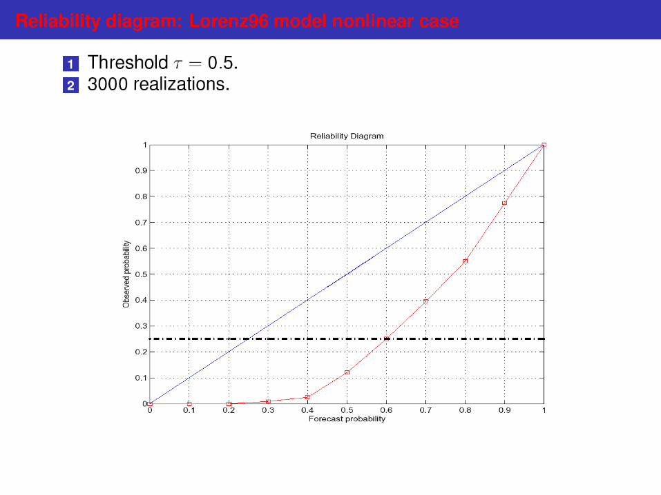
(Nonlinear) Lorenz’96 model

There is no (and there cannot be) a general objective test of bayesianity. We use here as a substitute the much weaker property of reliability.

Reliability. Statistical consistency between predicted probability of occurrence and observed frequency of occurrence (it rains 40% of the time in circumstances when I predict 40%-probability for rain).

Observed frequency of occurrence p‘(p) of event, given that it has been predicted to occur with probability p, must be equal to p.

For any p, p‘(p) = p

More generally, frequency distribution F‘(F) of reality, given that probability distribution F has been predicted for the state of the system, must be equal to F.

Reliability can be objectively assessed, provided a large enough sample of realizations of the estimation process is available.

Reliability diagramme, NCEP, event T850 > Tc - 4C, 2-day range,

Northern Atlantic Ocean, December 1998 - February 1999

Rank histograms, T850, Northern Atlantic, winter 1998-99

Top panels: ECMWF, bottom panels: NMC (from Candille, Doctoral Dissertation, 2003)

In both linear and nonlinear cases, size of ensembles Ne =30

Number of realizations of the process M =3000 and 7000 for Lorenz and Kuramoto-Sivashinsky respectively.

Non-gaussianity of the error, if model is kept linear, has no significant impact on scores.

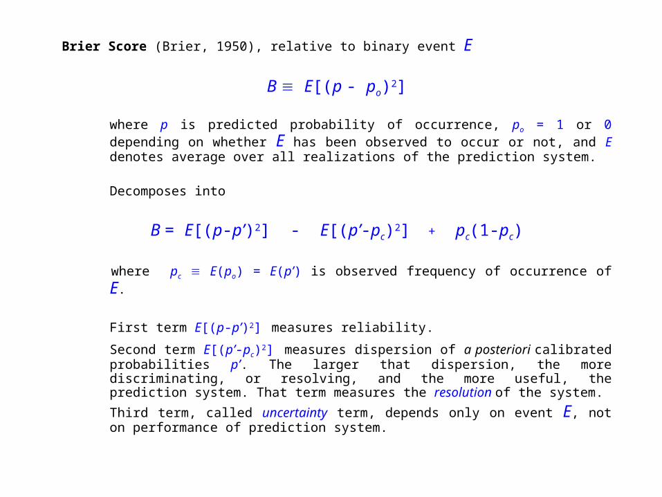
Brier Score (Brier, 1950), relative to binary event E

B E[(p - po)2]

where p is predicted probability of occurrence, po = 1 or 0 depending on whether E has been observed to occur or not, and E denotes average over all realizations of the prediction system.

Decomposes into

B = E[(p-p’)2] - E[(p’-pc)2] + pc(1-pc)

where pc E(po) = E(p’) is observed frequency of occurrence of E.

First term E[(p-p’)2] measures reliability.

Second term E[(p’-pc)2] measures dispersion of a posteriori calibrated probabilities p’. The larger that dispersion, the more discriminating, or resolving, and the more useful, the prediction system. That term measures the resolution of the system.

Third term, called uncertainty term, depends only on event E, not on performance of prediction system.

Reliability diagramme, NCEP, event T850 > Tc - 4C, 2-day range,

Northern Atlantic Ocean, December 1998 - February 1999

Brier Skill Score

BSS 1 - B/pc(1-pc)

(positively oriented)

and components

Brel E[(p-p’)2]/pc(1-pc)

Bres 1 - E[(p’-pc)2] /pc(1-pc)

(negatively oriented)

Very similar results obtained with the Kuramoto-Sivashinsky equation.

Preliminary conclusions

• In the linear case, ensemble variational assimilation produces, in agreement with theory, reliable estimates of the state of the system.

• Nonlinearity significantly degrades reliability (and therefore bayesianity) of variational assimilation ensembles. Resolution (i. e., capability of ensembles to reliably estimate a broad range of different probabilities of occurrence, is also degraded. Similar results (not shown) have been obtained with Particle Filter, which produces ensembles with low reliability.

Perspectives

• Perform further studies on physically more realistic dynamical models (shallow-water equations)

• Further comparison with performance Particle Filters, and with performance of Ensemble Kalman Filter.

Bayesian estimation (continued)

Consider again general situation

z = F(x, ) (1)

What if probability distribution for is not known, or known insufficiently for determining posterior bayesian probability distribution for x ?

Consider class C of all probability distributions for xithat are compatible with data (i. e., that are the bayesian posterior probability distribution for some choice of missing information on distribution for ). Then choose one distribution in C.

Frequent choice. Choose pdf p(x) which maximizes entropy

E -p(x) lnp(x) dx = - E [lnp(x)]

Maximum entropy (S. Losa). Least commiting choice

Bayesian estimation (continued)

In the case

z = x +

assuming that only expectation and covariance matrix S of are known, entropy-maximizing

probability distribution is gaussian distribution N [xa, Pa] defined above.

Question. How to quantify uncertainty ?

Through bounds, and then interval arithmetic, which carries the bounds through the computations

? That has probably been done. But if operator F-1, while existing, is unbounded, bounds are

infinite. Regularization can help here (but is it legitimate to use regularization only for

imposing bounds for which there is no physical justification ?).

‘Most-squares’ method presented by M. Meju.

Through probability distributions ? Probability distributions are very convenient for describing

uncertainty, especially when it comes to updating uncertainty through Bayes’ rule.

Jaynes, E. T. 2007, Probability Theory: The Logic of Science, Cambridge University Press.

Following an earlier work by Cox (1946), author posits a number of axioms that

any numerical function that measures ‘uncertainty’ must verify, and then finds

(maths is not trivial) that such an uncertainty function follows the rules of calculus

of probability.

Alternative approaches

- Dempster Shafer theory of evidence (Dempster, A. P., 1967, Annals of Math. Statistics, Shafer, G., 1976, A mathematical theory of evidence. Princeton Univ. Press). Introduces distinct notions of belief and plausibility.Has been used in remote observation of Earth surface parameters.

- Theory of possibility (link with fuzzy logic and fuzzy sets (Zadeh, L. A., 1978, Fuzzy Sets and Systems)

SIAM Activity Group on Uncertainty Quantification (http://www.siam.org/activity/uq/)

Statistical and Applied Mathematical Sciences Institute ((SAMSI) 2011-12 Program on Uncertainty Quantification (http://www.samsi.info/programs/2011-12-program-uncertainty-quantification)

- A few problems to be solved

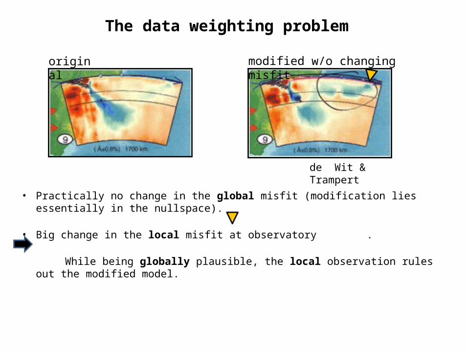
• Practically no change in the global misfit (modification lies essentially in the nullspace).

• Big change in the local misfit at observatory .

While being globally plausible, the local observation rules out the modified model.

original modified w/o changing misfit

de Wit & Trampert

The data weighting problem

original modified w/o changing misfit

de Wit & Trampert

• Practically no change in the global misfit (modification lies essentially in the nullspace).

• Big change in the local misfit at observatory .

While being globally plausible, the local observation rules out the modified model.

Can uncertainties be based on one single scalar misfit measure?

Can we attach more significance to observatory without becoming un-Bayesian?

What do we do with all the other observatories that may claim to be as important as observatory ?

The data weighting problem

- How to represent, or even define, uncertainty ?

- How to objectively evaluate estimates of uncertainty (requires very large validation sets, that may not be available for solid Earth) ?

- Identification and validation of errors in ‘models’ (in the sense of statements of relevant physical laws)

Announcement

International Conference on Ensemble Methods in Geophysical Sciences

Supported by World Meteorological Organization, Météo-France, Agence Nationale de la Recherche (France)

Dates and location : 12-16 November 2012, Toulouse, France

Forum for study of all aspects of ensemble methods for estimation of state of geophysical systems (atmosphere, ocean, solid earth, …), in particular in assimilation of observations and prediction : theory, algorithmic implementation, practical applications, evaluation, …

Scientific Organizing Committee is being set up. Announcement will be widely circulated in coming weeks.

If interested, send email to talagrand@lmd.ens.fr