Nationaal Lucht- en Ruimtevaartlaboratorium

National Aerospace Laborator y NLR

NLR-TP-98448

A pilot model for helicopter manoeuvres

J. van der Vorst

������������������������������������ ��� �� ������������������������ �� ������������������������ �� ������������������������ �� ���������������������

�������� ��� �� ���������� ���

����������

���������������� �������������������������������� �������������������������������� �������������������������������� ����������������

�� ��� �� ��

This report is based on a presentation held at the 24th European Rotorcraft Forum,Marseille, France, 15-17 September 1998

The contents of this report may be cited on condition that full credit is given to NLR and

the author.

Division: FlightIssued: January 2001Classification of title: Unclassified

-3-NLR-TP-98448

Summary

Since helicopter handling qualities are becoming more and more important, there is a need for

tools to analyse these qualities. The primary goal of the research described in this paper was the

development of a pilot model with which offline simulations can be performed of “piloted”

helicopter manoeuvres, such as ADS33D Flight Test Manoeuvres. In order to develop such a

pilot model, a literature study was performed about the types of pilot models available.

Furthermore, to determine the underlying structure of the controlling and guiding process, pilots

were interviewed about how they executed certain manoeuvres and discerned the various phases

within a manoeuvring task.

The control model structure contains a so-called “high-level”, “mid-level” and a “low-level”

structure. These levels are associated with navigation (long-term course & altitude control),

guidance (mid-term speed and position control) and stabilisation (short-term attitude control)

respectively. These sub-models were implemented in sequence. For the navigation module use

was made of specific user-defined directives, mostly obtained from questionnaires. For the

guidance module PID-controllers per control axis were developed. For the stabilisation module

the Structural Pilot Model was applied containing typical human structural elements. The

helicopter model used is a 6 DOF non-linear model, using closed-form equations for the main

rotor. The BO-105 helicopter has been modelled, since much flight test data from DLR was

available to develop and tune the model.

The pilot/helicopter model was validated by comparing simulation results with actual flight test

data. Two ADS33 manoeuvres were simulated, one longitudinal manoeuvre, the accel/decel,

and one lateral manoeuvre, the sidestep. The simulation responses compared quite well with the

flight test data. Off-axis responses were not predicted quite well, however, these might be

improved by including feed-forward (anticipation) in the pilot model and by improving the

fidelity of the helicopter model.

Feasibility of the suggested model structure has been demonstrated. However, implementation

of the manoeuvre to be flown required extensive piloting task analysis. Tuning of the model

using flight data is required to match the model parameters in order to derive predictive

capability.

There are several future applications for the model. The complete model structure lends itself to

help build a pilot model that allows handling quality ratings (like “Cooper-Harper”) to be given.

The model may also shed light on the fidelity of the cues provided by a flight simulator.

-4-NLR-TP-98448

Contents

Summary 3

Notation 5

1 Introduction 7

2 Literature study 8

3 Structure of the pilot model 11

4 Helicopter model 14

5 Simulation results of the helicopter/pilot model 15

5.1 ADS33D accel/decel manoeuvre 15

5.2 ADS33D sidestep manoeuvre 17

6 Conclusions and recommendations 19

6.1 Conclusions 19

6.2 Recommendations 20

6.3 Acknowledgements 20

7 References 21

(25 pages in total)

-5-NLR-TP-98448

Notation

Symbols

h height (m)

h� dh/dt (m/s)

H transfer function

K gain

Ke equivalent pilot gain for SPM

K1 proprioceptive feedback gain for SPM

Y transfer function

ε rel. amount of integral action for SPM (-)

θ pitch attitude (deg or rad)

τ0 time delay (s)

ω frequency (rad/s)

ωc crossover frequency (rad/s)

ωn natural frequency (rad/s)

ζ damping ratio (-)

Subscripts

C controlled element (=helicopter)

h height

int_h integral of height

NM Neuro Muscular

OL Open Loop

P Pilot

PF Proprioceptive Feedback

req required

Abbreviations

COM Crossover Model

FTM (ADS33D) Flight Test Manoeuvre

HQR Handling Qualities Rating

OCM Optimal Control Model

PID Proportional-Integral-Derivative

SPM Structural Pilot Model

-6-NLR-TP-98448

This page is intentionally left blank

-7-NLR-TP-98448

1 Introduction

Since helicopters have inherently poor handling qualities, analysis of these qualities is of major

importance. In recent years a modern set of handling qualities requirements and criteria,

ADS33D, have been set up by the US Army (Ref. 2). It uses, among other things, so called

Flight Test Manoeuvres (FTMs) for assessing handling qualities of helicopters.

It would be interesting to fly these FTMs with a helicopter simulation program. This would

either require a human or a pilot model to ‘fly’ the simulation. The disadvantage of a human is

in the area of repeatability. If the human flies the same manoeuvre twice, there will be at best

two slightly different manoeuvres. A mathematical pilot model does not have this disadvantage.

Moreover, for a human pilot expensive real-time simulation is required, whereas a pilot-model

can be simulated off-line.

Such a model will lead to a clearer insight into the execution of manoeuvres by human pilots.

Ultimately the model could generate pilot handling qualities ratings. Since cues for determining

the different phases in each manoeuvre are essential in the pilot model, this will also allow the

fidelity of cues, provided by a flight simulator, to be investigated analytically.

Therefore, the goal of this research is to develop a pilot-manoeuvre model, with human pilot

aspects, for flying prescribed manoeuvres with a helicopter.

First, a literature study was performed to investigate existing pilot models. Next, a non-linear,

six degrees-of-freedom helicopter simulation was created, to be used as a tool in developing and

testing the pilot-manoeuvre model. A structure for the pilot model was defined and

implemented. With this pilot/helicopter model two FTMs were simulated, the accel/decel and

the sidestep. The helicopter modelled is the Eurocopter BO-105, since DLR flight test data of

ADS33D Flight Test Manoeuvres was available for this type of helicopter.

-8-NLR-TP-98448

2 Literature study

A number of pilot models can be found in literature. One of the earliest models is the Crossover

Model (Ref. 3). According to this model the pilot will adjust his control behaviour to the

dynamics of the system he is controlling, such that the open-loop characteristics of the

combination of pilot and controlled system can be described by (Ref. 3):

HOL (ω) = Hp(ω)⋅Hc(ω) = ω

⋅ω ωτ−

j

e ejc

In this equation ωc is the crossover frequency, at which the amplitude of HOL equals one. The

time constant τe is the equivalent time delay due to information processing by the pilot.

The advantages of the Crossover Model are that it works well, certainly well enough for

engineering applications and that it is simple. The disadvantages are that it is only valid around

the crossover frequency and that it is only valid for compensatory tracking tasks.

Another model is the Optimal Control Model (OCM). The main assumption of the Optimal

Control Model is that a well-trained, well-motivated human operator behaves in an optimal

manner, subject to his inherent limitations and to the requirements of the control task (Ref. 4).

An advantage of the Optimal Control Model is that it can be used for a wide range of

frequencies (as opposed to the Crossover Model). Furthermore the OCM is more suited for

situations in which there is very limited information on pilot behaviour: the OCM gives

information on which cues are important in the manoeuvre.

On the other hand the disadvantage is that the translation of a practical situation to theoretical

OCM parameters is not simple. This often leads to a large number of assumptions to be

satisfied. Furthermore, the OCM parameters cannot be estimated directly from experimental

data (this can be done for the Crossover Model).

Neuromuscular SystemCentral Nervous System

-

+

+

+

-

+Ke e-τ0·s Yc

YNM

uδ

YPF

um

K1

(s+a)n

command

heliresponse

ε/s

2nn

2

2n

s2s ω+ζω+

ω

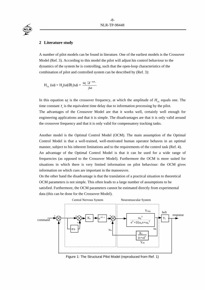
Figure 1: The Structural Pilot Model (reproduced from Ref. 1)

-9-NLR-TP-98448

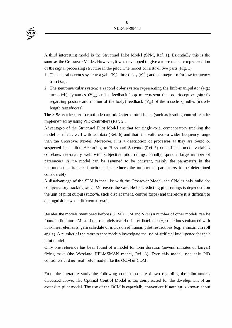
A third interesting model is the Structural Pilot Model (SPM, Ref. 1). Essentially this is the

same as the Crossover Model. However, it was developed to give a more realistic representation

of the signal processing structure in the pilot. The model consists of two parts (Fig. 1):

1. The central nervous system: a gain (Ke), time delay (e-τ0s) and an integrator for low frequency

trim (ε/s).

2. The neuromuscular system: a second order system representing the limb-manipulator (e.g.:

arm-stick) dynamics (YNM) and a feedback loop to represent the proprioceptive (signals

regarding posture and motion of the body) feedback (YPF) of the muscle spindles (muscle

length transducers).

The SPM can be used for attitude control. Outer control loops (such as heading control) can be

implemented by using PID-controllers (Ref. 5).

Advantages of the Structural Pilot Model are that for single-axis, compensatory tracking the

model correlates well with test data (Ref. 6) and that it is valid over a wider frequency range

than the Crossover Model. Moreover, it is a description of processes as they are found or

suspected in a pilot. According to Hess and Sunyoto (Ref. 7) one of the model variables

correlates reasonably well with subjective pilot ratings. Finally, quite a large number of

parameters in the model can be assumed to be constant, mainly the parameters in the

neuromuscular transfer function. This reduces the number of parameters to be determined

considerably.

A disadvantage of the SPM is that like with the Crossover Model, the SPM is only valid for

compensatory tracking tasks. Moreover, the variable for predicting pilot ratings is dependent on

the unit of pilot output (stick-%, stick displacement, control force) and therefore it is difficult to

distinguish between different aircraft.

Besides the models mentioned before (COM, OCM and SPM) a number of other models can be

found in literature. Most of these models use classic feedback theory, sometimes enhanced with

non-linear elements, gain schedule or inclusion of human pilot restrictions (e.g. a maximum roll

angle). A number of the more recent models investigate the use of artificial intelligence for their

pilot model.

Only one reference has been found of a model for long duration (several minutes or longer)

flying tasks (the Westland HELMSMAN model, Ref. 8). Even this model uses only PID

controllers and no ‘real’ pilot model like the OCM or COM.

From the literature study the following conclusions are drawn regarding the pilot-models

discussed above. The Optimal Control Model is too complicated for the development of an

extensive pilot model. The use of the OCM is especially convenient if nothing is known about

-10-NLR-TP-98448

how to fly a manoeuvre. That is not the case in this report, the manoeuvres to be flown are well

defined in the ADS-33 document.

The Crossover Model is simple, not over-parameterised and should be applicable.

The Structural Pilot Model is essentially the same as the Crossover Model, however more

interesting, since it reflects the information processing in the human body. Therefore the SPM

was applied in this research.

Since the pilot-manoeuvre model has to be capable of flying prescribed manoeuvres, two

example ADS33D Flight Test Manoeuvres have been selected: the accel/decel and the sidestep.

The reasons for choosing these are:

1. Both are aggressive manoeuvres, so they will induce much cross coupling and will require

helicopter and pilot operating at the limits of capability.

2. Both manoeuvres vary in flight condition from hover to forward/sideward flight, so the

rapidly varying handling qualities of the helicopter will play a role.

3. The accel/decel is mainly a longitudinal manoeuvre, while the sidestep is a lateral

manoeuvre. In both manoeuvres, apart from longitudinal and lateral cyclic, the collective

and pedal controls are important as well. By choosing these manoeuvres, all control axes are

represented.

According to the ADS33D document (Ref. 2), the accel/decel manoeuvre starts from hover,

then a high performance (fast) acceleration is performed to a speed of 50 knots, followed by a

high performance (fast) deceleration ending in a hover again. During the manoeuvre the

altitude, heading and lateral track have to be maintained within certain limits. The length of the

course depends on the performance of the helicopter it is flown with.

The sidestep manoeuvre starts from a hover as well. An aggressive lateral translation is

performed with a bank angle of at least 25 degrees. Upon reaching the maximum allowable

lateral airspeed (within 5 knots), or 45 knots, an aggressive deceleration back to hover is

performed with a bank angle of at least 30 degrees. After hovering for 5 seconds the manoeuvre

is repeated in the opposite direction. During the manoeuvre the height, heading and longitudinal

track have to be maintained within certain limits.

-11-NLR-TP-98448

3 Structure of the pilot model

Before implementing the pilot model in a program, a clear structure has to be defined. This is

based on the three piloting functions as distinguished by Padfield (Ref. 9):

1. Navigation (Long-term course and altitude control)

2. Guidance (Mid-term velocity or position control)

3. Stabilisation (Short-term attitude control)

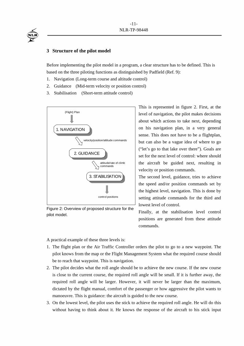
This is represented in figure 2. First, at the

level of navigation, the pilot makes decisions

about which actions to take next, depending

on his navigation plan, in a very general

sense. This does not have to be a flightplan,

but can also be a vague idea of where to go

(“let’s go to that lake over there”). Goals are

set for the next level of control: where should

the aircraft be guided next, resulting in

velocity or position commands.

The second level, guidance, tries to achieve

the speed and/or position commands set by

the highest level, navigation. This is done by

setting attitude commands for the third and

lowest level of control.

Finally, at the stabilisation level control

positions are generated from these attitude

commands.

A practical example of these three levels is:

1. The flight plan or the Air Traffic Controller orders the pilot to go to a new waypoint. The

pilot knows from the map or the Flight Management System what the required course should

be to reach that waypoint. This is navigation.

2. The pilot decides what the roll angle should be to achieve the new course. If the new course

is close to the current course, the required roll angle will be small. If it is further away, the

required roll angle will be larger. However, it will never be larger than the maximum,

dictated by the flight manual, comfort of the passenger or how aggressive the pilot wants to

manoeuvre. This is guidance: the aircraft is guided to the new course.

3. On the lowest level, the pilot uses the stick to achieve the required roll angle. He will do this

without having to think about it. He knows the response of the aircraft to his stick input

1. NAVIGAT ION

2. GUIDANCE

3. ST ABILISAT ION

velocity/position/altitude commands

attitude/rate of climbcommands

control positions

(Flight) Plan

Figure 2: Overview of proposed structure for the

pilot model.

-12-NLR-TP-98448

through training and experience. This is stabilisation: the aircraft is stabilised around the

required attitude.

Implementation of the structure

Navigation

The navigation level involves conscious decisions by the pilot regarding the action next to be

taken. It would require artificial intelligence to automate this level, which is complicated.

Therefore, user-defined directives are used. This means that the user of the pilot/helicopter

simulation program will have to divide the manoeuvre into phases (e.g.: hover, acceleration,

deceleration, etc.). For each of these phases he has to decide which intermediate (guidance)

goals have to be achieved (e.g.: heading, speed, altitude commands). The user has to do this by

thorough analysis of the manoeuvre. Three sources have been used in this research. First of all,

the ADS33D document gives a good initial impression of how the manoeuvre has to be flown.

Secondly, pilots were interviewed about how they fly the manoeuvre and which phases they

discern. Finally, DLR flight test data was available to inspect closely how a manoeuvre is

flown. For the accel/decel manoeuvre this analysis resulted in the following five phases:

1. Initial hover

2. Acceleration

3. Flare deceleration

4. Collective pull deceleration

5. Final hover

The sidestep was divided into seven phases:

1. Initial hover

2. First sideward acceleration

3. Sideward deceleration

4. Intermediate hover

5. Second sideward accel. (opposite direction)

6. Sideward deceleration

7. Final hover

Guidance

The goals generated by the navigation level are fed to the next level, guidance. These goals are

transformed into attitude commands, through PID-controllers. The gains of the PID-controllers

were determined manually.

An example of such a PID controller is the altitude hold by controlling pitch attitude (which is

in its turn controlled by the longitudinal SPM):

-13-NLR-TP-98448

hKdthhKhhK hdotreqhreqhreq�⋅+−+−⋅=θ ∫ )()( int_

Examples of PID controllers are altitude hold with collective, altitude hold with longitudinal

cyclic, longitudinal position hold, lateral position hold, heading hold, etc.

Stabilisation

The attitude commands from the guidance level are fed into the stabilisation level, consisting of

the Structural Pilot Model mentioned before. This stabilisation level outputs stick positions,

which are fed into the helicopter simulation program.

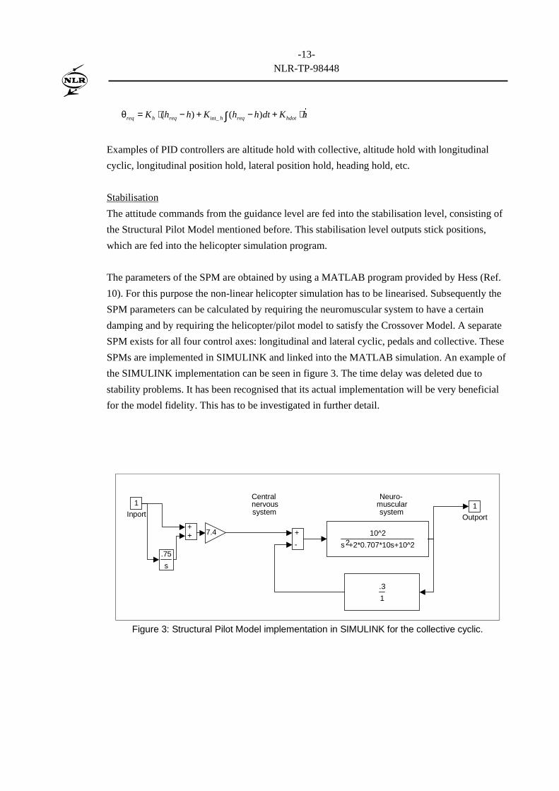
The parameters of the SPM are obtained by using a MATLAB program provided by Hess (Ref.

10). For this purpose the non-linear helicopter simulation has to be linearised. Subsequently the

SPM parameters can be calculated by requiring the neuromuscular system to have a certain

damping and by requiring the helicopter/pilot model to satisfy the Crossover Model. A separate

SPM exists for all four control axes: longitudinal and lateral cyclic, pedals and collective. These

SPMs are implemented in SIMULINK and linked into the MATLAB simulation. An example of

the SIMULINK implementation can be seen in figure 3. The time delay was deleted due to

stability problems. It has been recognised that its actual implementation will be very beneficial

for the model fidelity. This has to be investigated in further detail.

Centralnervoussystem

Neuro-muscularsystem

+

-

++ 7.4

.3

1

10^2

s +2*0.707*10s+10^22

.75

s

1

Inport1

Outport

Figure 3: Structural Pilot Model implementation in SIMULINK for the collective cyclic.

-14-NLR-TP-98448

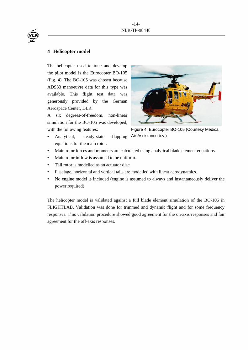
4 Helicopter model

The helicopter used to tune and develop

the pilot model is the Eurocopter BO-105

(Fig. 4). The BO-105 was chosen because

ADS33 manoeuvre data for this type was

available. This flight test data was

generously provided by the German

Aerospace Center, DLR.

A six degrees-of-freedom, non-linear

simulation for the BO-105 was developed,

with the following features:

• Analytical, steady-state flapping

equations for the main rotor.

• Main rotor forces and moments are calculated using analytical blade element equations.

• Main rotor inflow is assumed to be uniform.

• Tail rotor is modelled as an actuator disc.

• Fuselage, horizontal and vertical tails are modelled with linear aerodynamics.

• No engine model is included (engine is assumed to always and instantaneously deliver the

power required).

The helicopter model is validated against a full blade element simulation of the BO-105 in

FLIGHTLAB. Validation was done for trimmed and dynamic flight and for some frequency

responses. This validation procedure showed good agreement for the on-axis responses and fair

agreement for the off-axis responses.

Figure 4: Eurocopter BO-105 (Courtesy Medical

Air Assistance b.v.)

-15-NLR-TP-98448

5 Simulation results of the helicopter/pilot model

The simulation results have been compared to DLR flight test data. The simulated manoeuvre

and real flight test manoeuvre are not exactly the same. These differences are either due to a

difference in implementation (the flight test pilot and the pilot model use a slightly different

technique) or due to differences in the helicopter modelling (the flight test pilot and the pilot

model fly slightly different helicopters).

In all the figures there are vertical, dashed lines with a number on top. These denote the start of

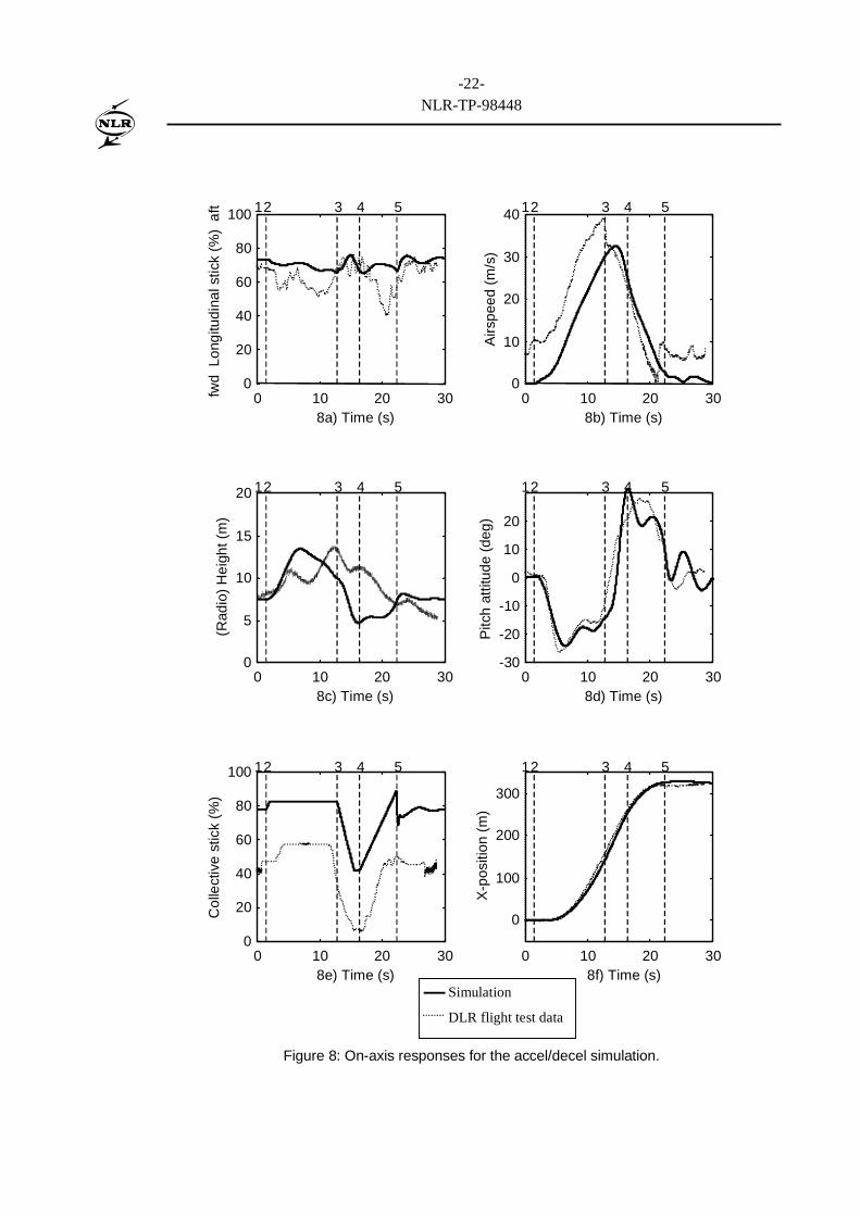
the different phases of the manoeuvre. So, the line with number 5 on top indicates the starting

time of phase 5.

5.1 ADS33D accel/decel manoeuvre

The first simulated manoeuvre was the ADS33D accel/decel. In figure 8 the on-axis response

parameters can be found. Graph 8a shows longitudinal cyclic, which is closely related to the

pitch attitude in graph 8d. Clearly simulation and flight test data have the same trend. Initially

the helicopter is pushed nose down to accelerate. Then it is pulled up a bit, followed by more

nose down cyclic to correct for the increasing airspeed. In phase 3 (deceleration) the helicopter

is rotated nose up to a maximum pitch attitude of 32°. Subsequently it is pushed over into a

hover. In phases 3 and 4 it was very difficult to maintain height in the simulation. Graph 8b

shows the airspeed. Flight test data starts at 8 m/s, probably due to the airspeed measurement

probe being in the downwash of the main rotor. Collective is shown in graph 8e. In the

simulation during phases 2, 3 and 4 the collective is not controlled by the Structural Pilot

Model. It is constant (phase 2) or has a fixed rate (phases 3 and 4). This rate determines the

aggression for performing the manoeuvre. When the pilot pulls collective aggressively, a fast

acceleration is the result. In the simulation, the rate has been adapted to match the flight test

data.

At the start of phase 5 collective is used to recover to the required height (7.5 m). This can be

seen in graph 8c. Initially the height increases due to the aggressive collective pull. When

decelerating, the helicopter has a strong tendency to sink, also in the flight test data. In the

simulation it was very difficult to control height in the deceleration. Finally graph 8f shows the

longitudinal position. The simulation lags behind flight test by about 15 meters. There is a little

overshoot (4 m) in position before stabilising into the hover. This is also seen in the flight test

data.

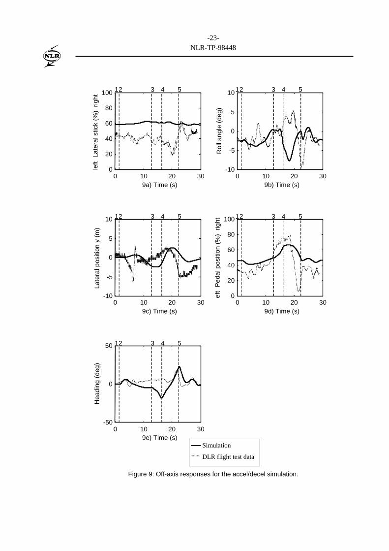
Figure 9 shows the off-axis responses for the accel/decel manoeuvre. In graph 9a the lateral

cyclic position can be found. The pilot model uses much less lateral cyclic input than the real

pilot. This is due to the rather simple helicopter model presently used. The resulting roll angles

are found in graph 9b. The magnitude is about the same for simulation and flight test. However,

-16-NLR-TP-98448

the trend is not identical. Especially in phase

4, the roll angle of the simulation is the

opposite of the flight test roll angle. This

might be a dynamic inflow effect, which is

not modelled. Graph 9c shows the resulting

lateral positions, which are of the same

magnitude as well. Graph 9d shows the

pedal position. Generally, the trend of the

simulation pedal position is the same as in

flight test. Graph 9e shows the resulting

heading angle. Again, the trend is about the

same. Around the start of phase 4, a large

deviation in heading of the simulation can

be seen. Probably, this indicates that the use of feedforward (anticipation) is required.

Ockier and Gollnick (Ref. 11) describe the results of ADS-33 flight-testing. About the

accel/decel manoeuvre they state that none of the test pilots achieved desired performance. This

is also apparent in the pilot model. The average HQR issued by the pilots was 5.3. Power and

rotor speed management were considered most difficult. The aggressive, 30° nose-up

deceleration, combined with the requirement to hover over a designated spot, was considered

problematic. This is visible in figure 9f, where both the real and simulated pilot make a slight

overshoot. Yaw control is problematic as well.

In general the accel/decel manoeuvre can be reasonably well ‘flown’ with the pilot model. It

could be improved by adding feedforward to improve heading control.

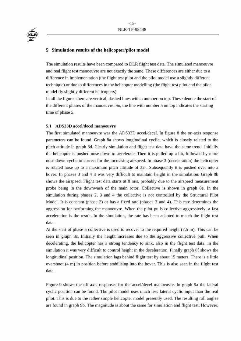
In figure 5 a three-dimensional representation of the simulated acceleration phase is shown. The

helicopter position and attitude is shown at 1-

second intervals. The helicopter noses down

and accelerates. Initially some height is

gained, due to the sudden collective pull.

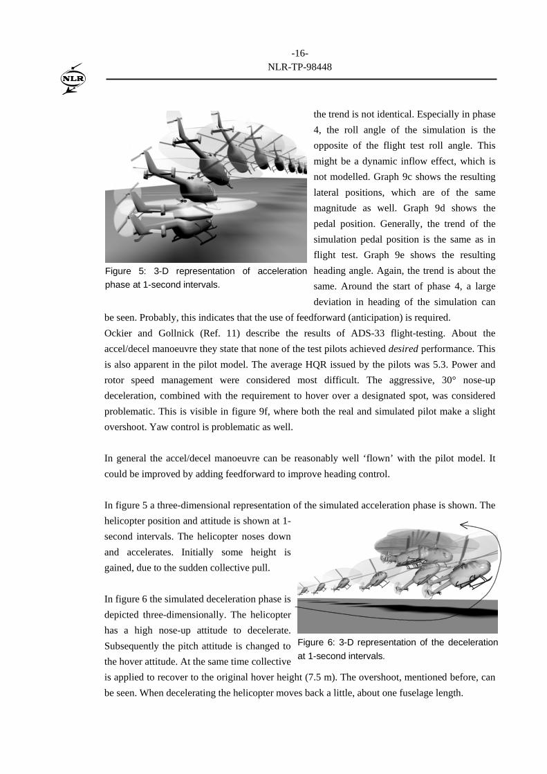
In figure 6 the simulated deceleration phase is

depicted three-dimensionally. The helicopter

has a high nose-up attitude to decelerate.

Subsequently the pitch attitude is changed to

the hover attitude. At the same time collective

is applied to recover to the original hover height (7.5 m). The overshoot, mentioned before, can

be seen. When decelerating the helicopter moves back a little, about one fuselage length.

Figure 5: 3-D representation of acceleration

phase at 1-second intervals.

Figure 6: 3-D representation of the deceleration

at 1-second intervals.

-17-NLR-TP-98448

5.2 ADS33D sidestep manoeuvre

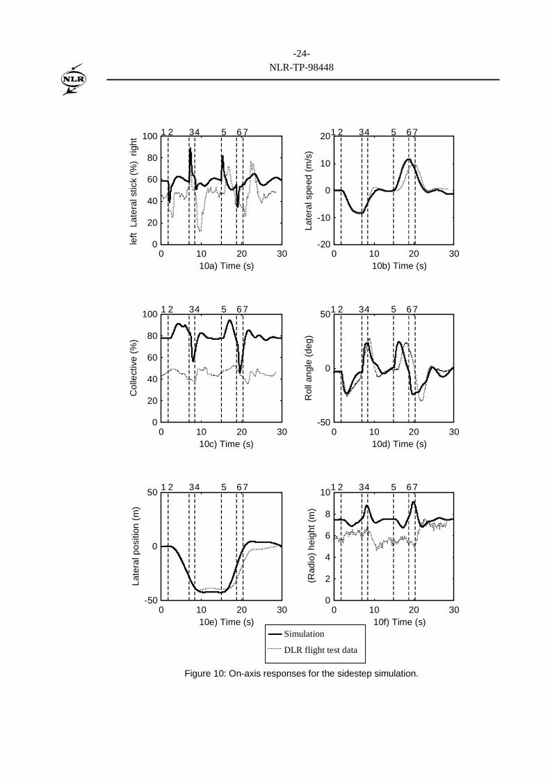
With the structure as defined before, the sidestep manoeuvre was simulated. Figure 10 and

figure 11 show the simulation results, together with the DLR flight test data.

Figure 10 shows the on-axis parameters for the sidestep manoeuvre. In graph 10a it can be seen

that the lateral stick position for the simulation follows the same trend as in flight test. The

resulting roll angle (graph 10d) is almost equal in both cases. The resulting lateral speed in

graph 10b is nearly identical as well. The lateral position is shown in graph 10e. Initially the

simulation position is equal to that in flight test. The intermediate hover positions are about 3

meters apart (from 9 to 17 seconds), on a total distance of 40 meters. The simulation starts the

return to the original hover position (phase 5) a little earlier. At the final hover (phase 7), the

simulation has some overshoot (4 m), while the flight test run shows some ‘undershoot’ (3 m).

Graph 10c shows the collective, necessary for maintaining height. Clearly the collective

movements are larger in the simulation. A possible reason for this might be the use of

feedforward and anticipation by the real pilot. He anticipates the rising of the helicopter at the

start of the deceleration. Therefore he will not correct when the helicopter descends just prior to

the deceleration, while the pilot model will do that. The use of anticipation and feedforward was

not investigated in this report. In graph 10f the resulting height can be seen. The height

deviations are slightly larger in the simulation, again an indication that anticipation is required.

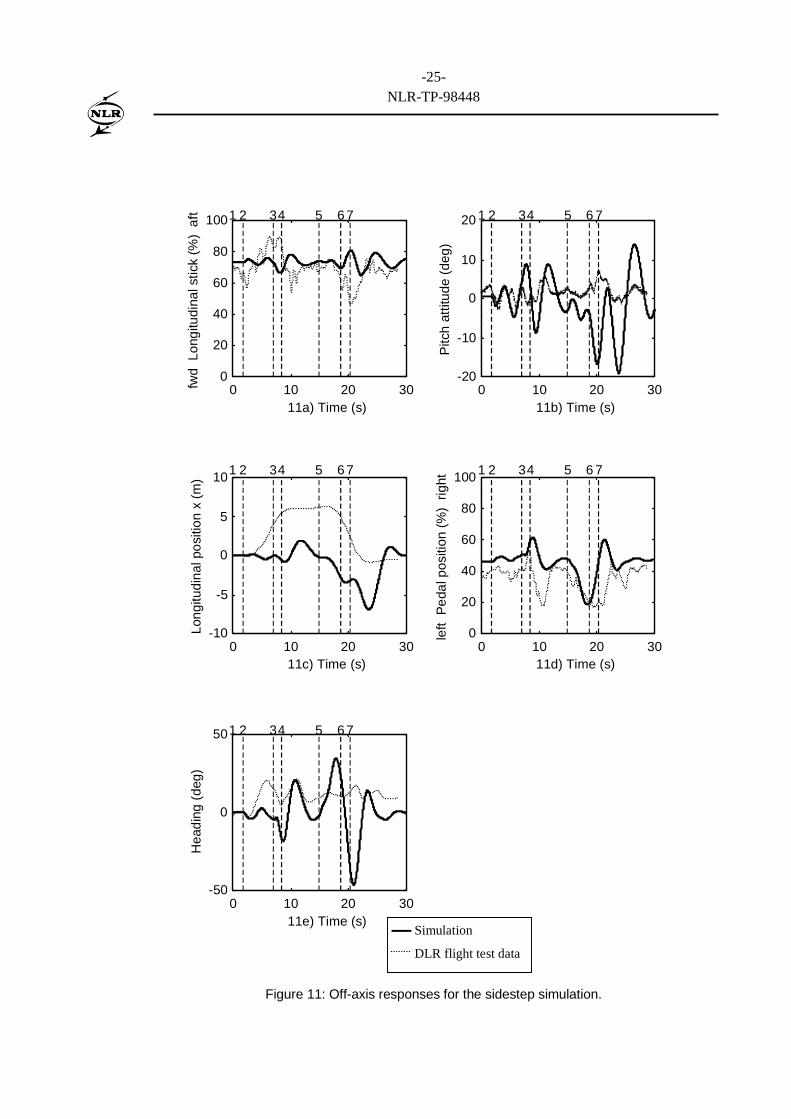
Figure 11 shows the off-axis parameters for the sidestep simulation. Graph 11a shows the

longitudinal stick input. Input in the simulation is much less than it was in the flight test. The

resulting pitch attitude is shown in graph 11b. The magnitude is the same for simulation and

flight test. However, the trend is not identical. Again, this is probably largely determined by

restrictions of the simple helicopter simulation. Graph 11c shows the longitudinal position. This

figure was obtained by integration of the accelerations. Due to inaccuracies in this

postprocessing procedure, the result contains a large component from the lateral acceleration

and is therefore unreliable. The position varies between +2 and -7 meters.

Graph 11d shows the pedal position required to maintain heading. Simulation and flight test

data show the same trend. In graph 11e very large heading deviations, from –45° to +35° can be

seen. This is definitely unacceptable in real flight. The flight test heading is calculated from the

yaw rate. The deviations are about ± 10°. The large deviation in the simulation indicates the use

of feedforward of collective to pedals (anticipation) is required. It shows as well that this

manoeuvre is very aggressive.

-18-NLR-TP-98448

Ockier and Vollnick (Ref. 11) describe pilot reactions for the sidestep manoeuvre. The average

HQR was 6.3, which is worse than the HQR for the accel/decel (HQR was 5.3) as mentioned

before. They write: “The sidestep manoeuvre is a very aggressive manoeuvre at the edge of the

BO-105s capabilities.” None of the pilots achieved desired performance. With this manoeuvre,

rotor speed/power control and yaw control was considered difficult. The simulation results are

in agreement with these observations.

In general it was harder to tune the sidestep manoeuvre than the accel/decel. The lateral

parameters are matched acceptably for the sidestep. For height and heading control anticipation

is required, so both collective and pedal inputs need feedforward. From the difference in the

pilots’ HQR and the difference in ease of implementation for the pilot model, we see that the

sidestep is a more aggressive manoeuvre than the accel/decel.

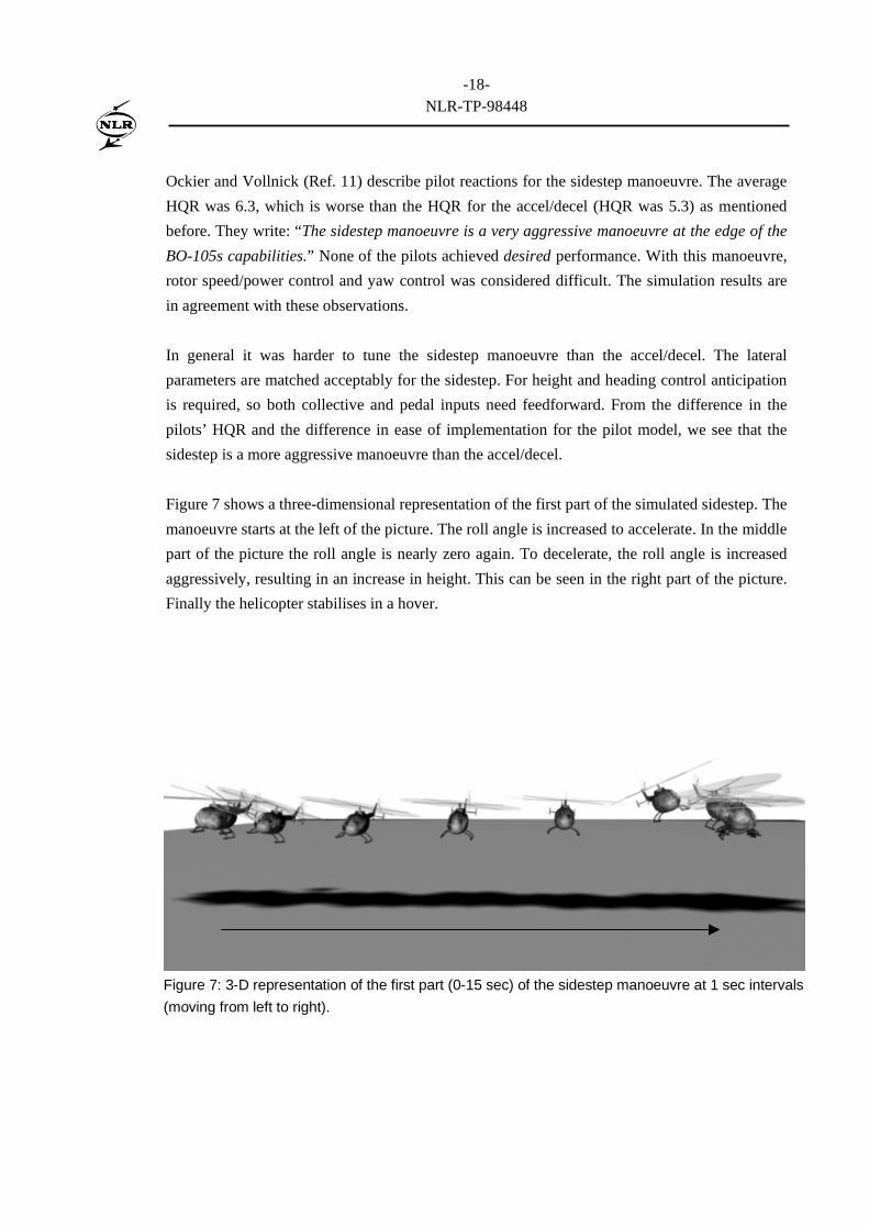
Figure 7 shows a three-dimensional representation of the first part of the simulated sidestep. The

manoeuvre starts at the left of the picture. The roll angle is increased to accelerate. In the middle

part of the picture the roll angle is nearly zero again. To decelerate, the roll angle is increased

aggressively, resulting in an increase in height. This can be seen in the right part of the picture.

Finally the helicopter stabilises in a hover.

Figure 7: 3-D representation of the first part (0-15 sec) of the sidestep manoeuvre at 1 sec intervals

(moving from left to right).

-19-NLR-TP-98448

6 Conclusions and recommendations

6.1 Conclusions

A pilot model has been developed, which is capable of flying prescribed manoeuvres with a

helicopter model. With respect to the pilot-manoeuvre model the following observations can be

made.

1. Feasibility of the pilot model for executing manoeuvres with a helicopter was demonstrated.

This was proven by the simulation of two ADS-33 flight test manoeuvres, the accel/decel

and sidestep manoeuvres. The simulations were tuned by comparison to flight test data,

provided by the German Aerospace Center (DLR).

2. Simulation of manoeuvres with the pilot model is possible. However, performing such a

simulation requires a lot of time consuming analysis and tuning.

3. The proposed structure (navigation, guidance and stabilisation functions) works well for the

simulation of the sidestep and accel/decel manoeuvres. It was slightly easier to tune the

accel/decel manoeuvre than the sidestep. Due to the aggressive nature of both manoeuvres,

timing is essential, just like it can be in real flight. Timing is reflected in the navigation

level of the pilot model.

4. The division of the accel/decel and sidestep manoeuvres in respectively 5 and 7 phases

appears to be valid.

5. The navigation level is considered the most important level. This level models the conscious

processes in the pilot. Therefore, the manoeuvre to be simulated should be thoroughly

analysed. Knowledge of piloting technique is required as well. It is this extensive analysis

that makes the program less suitable for quick analysis of pilot or helicopter behaviour in

new manoeuvres.

6. Generally the pilot model worked quite well. During aggressive parts of the simulated

manoeuvres, however, it appeared that addition of feedforward control would improve the

behaviour of the model. This applies particularly to heading control and height control.

7. The Structural Pilot Model (SPM), used for the lowest level stabilisation functions, works

well. Although fixed gains are used, based on the hover transfer functions, this does not

seriously impact the pilot model behaviour. Implementation of the SPM for the collective,

longitudinal cyclic and pedals was relatively straightforward. The lateral SPM however

showed slight oscillations and slow convergence to the required roll angle. This also had its

effect on guidance functions that used the lateral SPM. This could be either the helicopter

model or the pilot model.

-20-NLR-TP-98448

6.2 Recommendations

With regard to the pilot model the following recommendations are made.

1. To complete the Structural Pilot Model, its time delay (τ0) should be implemented. Thus, the

full effect of the SPM can be investigated and the human behaviour is implemented more

completely.

2. Presently, the SPM gain is determined using the transfer functions in hover only. Instead of

using a constant gain, a gain schedule could be used, depending on speed.

3. The possibility of predicting pilot opinion ratings should be examined. This was already

done by Hess, however, never for such a complete pilot model.

4. The pilot model was used assuming perfect observation. An investigation of the influence of

non-perfect observation would be interesting.

5. Feedforward control should be implemented to investigate the effect of anticipation in the

pilot model.

6. Combining the pilot model with a more complete helicopter simulation model than

currently used will provide a better basis for comparison with flight test data

6.3 Acknowledgements

This research was performed in the framework of a graduation project at the Faculty of

Aerospace Engineering at the Delft University of Technology. The author would like to thank

his mentors, both at the Faculty of Aerospace Engineering and at the National Aerospace

Laboratory (NLR).

-21-NLR-TP-98448

7 References

1. Hess, R.A., “Unified Theory for Aircraft Handling Qualities and Adverse Aircraft-PilotCoupling”. Journal of Guidance, Control and Dynamics, Vol. 20 No 6 1997, pp 1141-1148.

2. ADS-33D, “Handling Qualities Requirements for Military Rotorcraft”. U.S. Army Aviation

and Troop Command. St. Louis: July 1994.

3. McRuer, D.T.; Krendel, E.S., “Mathematical Models of Human Pilot Behavior.”

AGARDograph No. 188, Neuilly sur Seine: 1974.

4. Hosman, R.J.A.W., “Mens-Machine Systemen in Lucht- en Ruimtevaart” (Human Factors

in Aerospace, in Dutch, lecture notes). Delft: 1994, Faculty of Aerospace Engineering.

5. Hess, R.A., “Theory for Aircraft Handling Qualities Based Upon a Structural Pilot Model”

Journal of Guidance, Control and Dynamics, Vol. 12, No. 6, 1989, pp. 792-797.

6. Hess, R.A., “Structural Model of the Adaptive Human Pilot” Journal of Guidance, Control

and Dynamics, Vol. 3, No. 5 1980, pp 416-423.

7. Hess, R.A.; Sunyoto, I., “Toward a Unifying Theory for Aircraft Handling Qualities”

Journal of Guidance, Control and Dynamics, Vol. 8, No. 4 1985a, pp. 440-446.

8. Hamm, J., “The development of helicopter pilot models to control engineering simulations”

London: Royal Aeronautical Society, 1994.

9. Padfield, G.D., “Helicopter Flight Dynamics (The theory and application of flying qualities

and simulation modelling)” Oxford: Blackwell Science Ltd., 1996.

10. Hess, R.A.; Zeyada, Y., “PVD, Pilot/Vehicle Dynamics” Matlab program manual.

University of California, Davis, USA.

11. Ockier, C.J.; Gollnick, V., ADS-33 Flight Testing – Lessons Learned. AGARD Conference

Proceedings 592, Advances in Rotorcraft Technology, Ottawa, 27-30 May 1996. NATO:

AGARD-CP-592, April 1997.

-22-NLR-TP-98448

Figure 8: On-axis responses for the accel/decel simulation.

0 10 20 300

20

40

60

80

100

8a) Time (s)

fwd

Lon

gitu

dina

l stic

k (%

) a

ft 12 3 4 5

0 10 20 300

10

20

30

40

8b) Time (s)

Airs

peed

(m

/s)

0 10 20 300

5

10

15

20

8c) Time (s)

(Rad

io)

Hei

ght (

m)

0 10 20 30-30

-20

-10

0

10

20

8d) Time (s)

Pitc

h at

titud

e (d

eg)

0 10 20 300

20

40

60

80

100

8e) Time (s)

Col

lect

ive

stic

k (%

)

0 10 20 30

0

100

200

300

8f) Time (s)

X-p

ositi

on (

m)

12 3 4 5

12 3 4 5

12 3 4 5

12 3 4 5

12 3 4 5

Simulation

DLR flight test data

-23-NLR-TP-98448

Figure 9: Off-axis responses for the accel/decel simulation.

0 10 20 300

20

40

60

80

100

9a) Time (s)

left

Lat

eral

stic

k (%

) r

ight

0 10 20 30-10

-5

0

5

10

9b) Time (s)

Rol

l an

gle

(deg

)

0 10 20 30-10

-5

0

5

10

9c) Time (s)

Late

ral p

ositi

on y

(m

)

0 10 20 300

20

40

60

80

100

9d) Time (s)

eft

Pe

dal p

ositi

on (

%)

rig

ht

0 10 20 30-50

0

50

9e) Time (s)

Hea

din

g (

deg)

Simulation

DLR flight test data

12 3 4 5

12 3 4 5

12 3 4 5

12 3 4 5

12 3 4 5

-24-NLR-TP-98448

Figure 10: On-axis responses for the sidestep simulation.

0 10 20 300

20

40

60

80

100

10a) Time (s)

left

Lat

eral

stic

k (%

) r

ight

1 2 34 5 67

0 10 20 30-20

-10

0

10

20

10b) Time (s)

Late

ral s

peed

(m

/s)

0 10 20 300

20

40

60

80

100

10c) Time (s)

Col

lect

ive

(%)

0 10 20 30-50

0

50

10d) Time (s)

Rol

l an

gle

(deg

)

0 10 20 30-50

0

50

10e) Time (s)

Late

ral p

ositi

on (

m)

0 10 20 300

2

4

6

8

10

10f) Time (s)

(Rad

io)

heig

ht (

m)

Simulation

DLR flight test data

1 2 34 5 67

1 2 34 5 67 1 2 34 5 67

1 2 34 5 67 1 2 34 5 67

-25-NLR-TP-98448

0 10 20 300

20

40

60

80

100

11a) Time (s)

fwd

Lon

gitu

dina

l stic

k (%

) a

ft

0 10 20 30-20

-10

0

10

20

11b) Time (s)

Pitc

h at

titud

e (d

eg)

1 2 34 5 6 7

0 10 20 30-10

-5

0

5

10

11c) Time (s)

Long

itudi

nal p

osi

tion

x (m

)

0 10 20 300

20

40

60

80

100

11d) Time (s)

left

Pe

dal p

ositi

on (

%)

rig

ht

0 10 20 30-50

0

50

11e) Time (s)

Hea

din

g (

deg)

Simulation

DLR flight test data

1 2 34 5 67

1 2 34 5 6 71 2 34 5 67

1 2 34 5 67

Figure 11: Off-axis responses for the sidestep simulation.