Embed Size (px)
Citation preview

Kyoto University, Graduate School of Economics Research Project Center Discussion Paper Series
Default Effect Versus Active Decision: Evidence from a Field Experiment in Los Alamos
Wenjie Wang and Takanori Ida
Discussion Paper No. E-14-010
Research Project Center Graduate School of Economics
Kyoto University Yoshida-Hommachi, Sakyo-ku Kyoto City, 606-8501, Japan
September, 2014 June, 2017 Revised

Default Effect versus Active Decision: Evidence from a Field
Experiment in Los Alamos
Wenjie Wang∗ and Takanori Ida†
June 2017
Abstract
We examine how consumers respond to distinct combinations of preset defaults and subsequent economicincentives. A randomised controlled trial is implemented to investigate the demand reduction performanceof two electricity pricing programmes: opt-in and opt-out critical peak pricing. Both the intention-to-treatand the treatment-on-the-treated are more pronounced for customers assigned to the opt-in group. Thisresult suggests that the opt-in type active enrolment itself had an impact on customers’ subsequent behaviorand made them more responsive to the treatment intervention. Moreover, only the opt-in treatment hasspillover effects beyond the treatment time window. Our results, therefore, highlight the important differencebetween an active and a passive decision-making process.
JEL classification: C93, D12
Keywords: Field Experiment, Default Effect, Opt-in, Opt-out, Price Elasticity
∗Graduate School of Social Sciences, Hiroshima University, Japan. E-mail address: [email protected].†Corresponding author. Graduate School of Economics, Kyoto University. Yoshida-Honmachi, Sakyo, Kyoto, 606-
8501, Japan. Tel: +81-75-753-3477. E-mail address: [email protected].
1

1 Introduction
Decisions by default have become an important issue in behavioural economics and public pol-
icy (Johnson and Goldstein, 2013). We take an example from employees’ decisions on a 401(k)
retirement savings plan (Madrian and Shea, 2001). When employees must opt into the plan,
fewer than half enrol on their own. However, when they are automatically enrolled, few em-
ployees choose to opt out, resulting in close to 100% enrolment. A voluminous literature now
documents the successful applications of default effects, including retirement saving (Madrian
and Shea, 2001; Choi et al., 2002; Thaler and Benartzi, 2004; Chetty et al., 2014), organ dona-
tion (Spital, 1995; Johnson and Goldstein, 2003; Abadie and Gay, 2006), influenza vaccination
(Chapman et al., 2010), contractual choice in health clubs (DellaVigna and Malmendier, 2006),
and car insurance plan choices (Johnson et al., 1993). Most of these studies advocate for policies
with opt-out defaults (i.e. automatic enrolment defaults).
However, we emphasise in this paper that, in many situations, the calculation of an optimal
default may not be straightforward because the welfare impact on consumers could depend
not only on their initial choices but also on their subsequent behaviors after the enrolment.
Indeed, the high enrolment rate is by itself a powerful outcome in the saving literature (and
the literature cited above) because the enrolment automatically changes consumers’ choices
in a direction that is considered desirable by the policy maker. In contrast, there are also
many situations that enrolled consumers must demonstrate active subsequent behaviors for the
programme to be effective. Here, we encounter a trade-off. On the one hand, the option to
opt into an intervention may result in a limited number of participants, while the subsequent
outcomes for these participants may be large because of the attention triggered by the active
decision-making process. On the other hand, an opt-out default typically leads to extremely
high participation in the first stage, while the subsequent outcomes might be relatively small
across a large number of participants.
Therefore, the answer to the issue of optimal default options could be rather unclear, and
the related empirical evidence remains sparse, particularly evidence obtained from framed field
experiments. In an effort to bridge this gap, we implement a randomised experiment in Los
Alamos County (LAC), New Mexico, United States. Our primary data are high-frequency data
2
on household electricity consumption. The treatments are based on a popular dynamic electric-
ity pricing programme, namely critical peak pricing (CPP), which pre-commits households to
a high marginal price of electricity during peak demand hours. We randomly assign households
to one of three groups: 1) an opt-in CPP group, 2) an opt-out CPP group, and 3) a control
group. Note that the interventions in our experiment is relatively more complicated than those
in the retirement saving literature. In fact, our design can be regarded as a ‘two-stage’ policy
composed of a default-based enrolment process in the first stage of the experiment and price-
based incentives in the second stage. Under such experimental design, the eventual impact of
the policy will depend on how these factors interact with each other. For example, although
inertia may result in high participation in the first stage, customers’ attention and effort may
play a central role in the outcome of the second stage.
We present several findings from the experiment. First, the customer enrolment rate is
97.2% for the opt-out CPP group and 63.8% for the opt-in CPP group. We note that the
opt-in enrolment rate is relatively high compared with similar dynamic pricing programmes
(Potter et al., 2014). The high opt-in rate is particularly important to an experiment with
first-stage defaults and second-stage interventions because it helps identify the distinct effects
of opt-in and opt-out defaults on the subsequent outcomes. To the best of our knowledge, our
field experiment is among the first to identify such difference, which could be very hard to
capture if the opt-in enrolment rate is too low.
Second, we estimate the intention-to-treat (ITT) and treatment-on-the-treated (TOT) for
each treatment group, and the estimation results suggest that the opt-in default itself may
have made customers more responsive, reducing more electricity consumption during the event
period. In particular, the ITT captures the average causal effect of the treatment group as a
whole, and thus informs us of the overall policy outcome. We find that although the opt-in
enrolment rate is relatively low, the estimated ITT of opt-in CPP customers shows an average
percentage reduction (9.8%) of on-peak usage higher than that of opt-out CPP customers
(5.8%). In addition, the TOT captures the average causal effect of the customers who actually
switched to the new dynamic pricing tariff (i.e. the compliers) in each treatment group. The
estimated TOTs of opt-in customers show percentage reductions as high as 14.7%, much higher
than those of opt-out customers (6.0%). The ITT and TOT results also allow us to deduce that
3

the net effect of active enrolment itself corresponds to an average percentage reduction larger
than 5.6% (i.e., 38% of the opt-in TOT) among customers who opt into the CPP programme.
Third, we find that among the two treatment groups, only the opt-in group has spillover
effects in the sense that it even generated significant consumption reductions during the time
window preceding and following peak hours (i.e. shoulder hours) on treatment days. This result
also suggests that opt-in customers were more attentive than opt-out customers, and highlights
the difference between active decision making (opt-in) and passive decision making (opt-out).
This paper contributes to the literature on default effects and optimal enrolment rules, which
so far has focused on the initial impact of preset defaults. In contrast, how do these defaults
affect subsequent behavior of programme participants has not been well studied. Here, we em-
phasise the importance of such investigation as distinct enrolment procedures may enhance or
offset consumers’ subsequent behaviors in distinct ways. We document an example in which the
opt-in default and related active decision-making process had a more profound impact on house-
holds’ subsequent behaviors than its opt-out counterpart, both within and beyond treatment
event periods. Our result, therefore, suggests that the design of policies with default options
should be approached with caution, and the potential interactions among various components
of the policies may play a central role in determining the optimal procedure. These findings
may have policy implications in many fields of public economics such as health insurance, cell
phone service, and energy conservation, where consumers’ initial attention and decisions on
plan choice may significantly affect their subsequent behaviors on utilisation.
Additionally, our paper contributes to research in energy economics. Non-varying retail
prices do not reflect the high marginal cost of electricity during peak demand periods and, thus,
result in one of the largest inefficiencies in electricity markets. It has been widely recognised
that dynamic pricing such as CPP provides a promising solution. Unlike most existing studies,
our experiment is conducted in a rather mild climate (the average maximum temperature of
LAC is 77.2◦F in summer), with low saturation of the central air conditioning (CAC) systems
(about 10%), and we find significant treatment effects even in such an environment.
The remainder of this paper is organised as follows. Section 2 describes our experimental
design, data, and customer compliance. Section 3 presents the main results of our study,
including the treatment effect estimation strategies and results, and we conclude in Section 4.
4

2 Research Design and Data
2.1 Experiment Overview
The randomised field experiment was conducted for households in LAC in 2013. The experi-
ment was implemented in collaboration with the Los Alamos Department of Public Utilities, the
Los Alamos National Laboratory, New Energy and Industrial Technology Development Orga-
nization, Toshiba and Itochu. Smart meters, which record households’ electricity consumption
at 15-minute intervals, were installed in all the 1,648 households residing in the areas of North
and Barranca Mesas in LAC; these households form the target of our recruitment activities.
The installation of the meter system was completed in September 2012, and participant
recruitment began in February 2013 (Figure 1 shows the timeline of the experiment). To recruit
households, the Los Alamos Department of Public Utilities held a neighbourhood meeting on
the introduction of the randomised experiment and sent details of the experiment by mail to
households. We offered households US$50 as a participation incentive for the summer season
and US$50 for the winter season. Additionally, US$80 was offered upon the completion of
customer survey questions. The recruitment process ended in April 2013, and we recruited 914
households to participate in our experiment, which was more than half the total number of
target households. Note that these participants were self-selected samples as were the samples
in previous studies for electricity pricing experiments (Wolak, 2010, 2011; Faruqui and Sergici,
2011; Jessoe and Rapson, 2014; Ito, Ida, and Tanaka, 2017). A total of 798 (87.3%) of these
participant households also responded to the customer survey questions.
We randomly assigned the participants into treatment and control groups, which we clarify
in Section 2.2. In May 2013, participants were notified of their group assignment by mail and e-
mail, and were given the opportunity to choose between the dynamic pricing rate and standard
LAC flat rate on an opt-in or opt-out basis. The development of the smart grid system (that
is, the community energy management system) was completed at the end of June, and it was
in charge of the collection of participants’ consumption data, transmission of pricing signals,
and calculation of participants’ economic incentives.
The experiment ran during the summer from July to September and during the winter from
December to February. Those who decided to use the dynamic pricing rates were subject to a
5

maximum of 15 event days (i.e. treatment days) during summer and a maximum of 15 event
days during winter. In addition, dynamic pricing event hours were designed to be from 4 pm to 7
pm on event days.1 Event days were defined as the weekdays when on-peak aggregate electricity
consumption strains the capacity of the grid. Specifically, for the summer experimental period,
treatment days were announced if the day-ahead forecast of the peak load in the system exceeded
13,400 kW and the day-ahead forecast of the maximum temperature exceeded 78.8◦F (26◦C).
For the winter season, treatment days were announced if the day-ahead forecast of the peak
load exceeded 13,000 kW and the day-ahead forecast of the minimum temperature was lower
than 42.8◦F (6◦C). As a result, the treatment groups experienced 14 event days in summer and
15 event days in winter. The process of the determination of event days is demonstrated in
Figure 2.
The primary data of our study consist of the 15-minute electricity consumption records,
including both the data on the customers who participated in the experiment and the data
on those who decided not to participate. We also collect household data from surveys and
temperature data from the National Climatic Data Center (NOAA 2013-2014).
2.2 Treatments and Randomised Group Assignment
The treatments of this study are based on a popular dynamic pricing tariff, in which the price
during the peak period on a small number of demand-response event days is set much higher
than the standard rate.2
1We chose 4 pm to 7 pm as the event hours because the experiment was implemented in a residential area where
electricity usage peaks in the evening.2Our experimental design also includes a peak time rebate (PTR) tariff, in which a customer is given a rebate if the
on-peak usage is lower than certain PTR baseline on event days. The PTR tariff is of interest, particularly to regulators
and the electric power industry, because it does not charge high prices during the event period and, thus, is more desirable
than the CPP tariff in terms of customer protection. However, it is not useful to our current goal of comparing policies
with the same economic incentive and different preset default options. Therefore, we focus on the study of the two
CPP-based treatments in this paper. Furthermore, although CPP is totally exogenous to customers, PTR is endogenous
because the PTR baseline for each customer is determined as a function of the customer’s own electricity consumption
during the previous week. It is thus difficult to compare directly the average treatment effects of the CPP groups with
those of the PTR group.
6

Table 1: Pricing Schemes
Tariffs Event Day Event Day Non-Event Day
On-Peak Off-Peak
Flat 9.52¢/kWh 9.52¢/kWh 9.52¢/kWh
CPP 75¢/kWh 7.77¢/kWh 7.77¢/kWh
Notes: This table reports the details of the two pricing schemes studied in the paper: the standard flat rate (‘Flat’ in
the table) and the CPP rate (‘CPP’ in the table). The term ‘On-Peak’ refers to the time period from 4 pm to 7 pm and
‘Off-Peak’ refers to the remaining time period of the day.
Critical Peak Pricing: CPP is a dynamic pricing form that combines a fixed price structure
(either the usual flat rate or a discounted rate) with occasional departures from the fixed tariff
when power demand is high. In our experiment, the CPP tariff pre-commits households to a
high marginal price of electricity between the hours of 4 pm and 7 pm on event days. At the
same time, households pay a discounted tariff for consumption during other hours. Specifically,
the standard retail tariff in LAC is 9.52 cents/kWh. During the dynamic pricing events, the
electricity price for CPP customers was raised by a factor of approximately eight compared
with the standard rate, namely 75 cents/kWh. However, these customers needed only pay a
discounted price of 7.77 cents/kWh for consumption during all the other time periods of the
experiment.3 Table 1 demonstrates the structure of the LAC standard flat rate and CPP rate.
We randomly assigned 733 participant households to one of three groups: control, opt-in
CPP, and opt-out CPP (see Figure 3 for the experimental design and group assignment); these
households form the sample for our ‘opt-in versus opt-out’ study.4 Some attrition occurred
3This discounted price was designed under the revenue neutrality condition, which guarantees that bills under the
standard flat rate and CPP rate would be the same, on average, if there were no price elasticity; that is, if the customer’s
consumption behaviour remains the same under the two alternative rates. County-level aggregate consumption data in
the summer and winter seasons of 2012 were used for the calculation of revenue neutrality.4The remaining 181 participants were randomly assigned to the PTR treatment group (3 of them moved or requested
to be removed from the study before the beginning of the summer experiment).
7

before the beginning of the summer experiment; 11 households (1.5%) either moved or requested
to be removed from the study. Additionally, some attrition occurred after the completion of
the summer experiment; six households (0.8%) did not participate in the winter experiment.
Because the attrition occurred at approximately the same rate in each group and is small
compared with the total number of participants, it is unlikely to significantly bias our estimates.
We describe the control and treatment groups in detail:5
1. Control Group: A total of 174 households were assigned to the control group. These
households were informed of their group assignment, and they were subject to the standard
LAC flat rate during the experimental period. The control group did not receive any dynamic
pricing signals.
2. Opt-in CPP Group: A total of 365 households were assigned to this treatment group.
These households were informed of their group assignment and were notified that their default
rate was the standard flat rate and that they needed to “opt in” actively to receive the dynamic
price signals and use the CPP rate during the event periods. To do so, they had to respond
to an e-mail or an SMS message from the utility department. We assigned relatively more
customers to this group because, based on the results in other experimental studies of dynamic
pricing, we expected that the actual customer enrolment rate would be much lower than the
enrolment rate for the other treatment group.
3. Opt-out CPP Group: A total of 183 households were assigned to the opt-out CPP
group. These households were informed of their group assignment and notified that their default
rate was the CPP rate. In addition, households were informed that to switch to the standard
flat rate, they needed to ‘opt out’ from the CPP rate by responding to an e-mail or an SMS
message from the utility department.
Table 2 presents the descriptive statistics of the on-peak and off-peak usage preceding the first
CPP event (9 days of 15-minute consumption data6) and appliance ownership for each group.
5The number of households in each group is as of the beginning of the summer experiment, excluding the 11 dropouts.6As illustrated in Figure 1, the development of the smart grid system was completed at the end of June 2013, and
it began the collection of household-level 15-minute consumption data from July 2013. As a result, we have 9 days
of 15-minute consumption data preceding the first CPP event; these data were used as baseline usage data in the
difference-in-difference regression that will be described below.
8

Each column shows the mean and standard deviation of these observable characteristics of
households by group. The columns ‘P-value’ report the p-values of t-statistics for the difference
in means between each treatment group and control group. Because of the random assignment
of the groups, none of the difference in means is statistically significant. This supports the
integrity of the randomization.
CPP customers in both the opt-in and the opt-out treatment groups were informed of the
event days by day-ahead and same-day notices via e-mail or SMS messages. By contrast, cus-
tomers who chose to use the standard flat rate did not receive any notice during the experiment.
The detail of the notice is as follows:
‘Price event mm/dd, Peak 4p-7p. CPP rate $0.75/kWh peak, $0.0777/kWh non-peak.’
In addition, an incentive system similar to those in Jessoe and Rapson (2014, p.1421) and
Wolak (2010, 2011) was applied in our experiment. Following these experiments, we trans-
mitted the experimental price incentives via an off-bill account, and this account was credited
with 50 points (i.e. the participation incentive) at the beginning of each season. During the
experimental period, the amount of incentives lost or earned7 by the household was subtracted
from or added to the account balance. At the end of the experiment, any balance remaining in
the account was the customers to keep (i.e. one point = US$1). Throughout the experiment,
CPP customers in both treatment groups were apprised of their points accrual in the same
manner through a series of messages delivered by e-mail or SMS:
‘Points on DR day (mm/dd) = X1. Cumulative = X2 including non-DR days = X3.’
Additionally, at the conclusion of each season, the system informed CPP customers of the
total points earned for that season:
“Total points you’ve earned for this season are X4.”
7It equals the difference between the LAC standard flat tariff and CPP tariff multiplied by the quantity of the
household’s actual usage.
9

Table 2: Summary Statistics
Control Opt-in CPP Opt-out CPP
Variables Mean Mean P-value Mean P-value Obs.
(S.D.) (S.D.) (S.D.)
Pre-event on-peak usage (kWh/h) 1.09 1.06 0.74 1.03 0.44 722
(0.77) (0.73) (0.66)
Pre-event off-peak usage (kWh/h) 0.82 0.79 0.41 0.81 0.78 722
(0.51) (0.50) (0.48)
Number of central ACs 0.12 0.10 0.55 0.08 0.31 596
(0.41) (0.32) (0.30)
Number of window-unit ACs 0.37 0.30 0.31 0.40 0.73 596
(0.72) (0.67) (0.77)
Number of space heaters 0.66 0.60 0.48 0.68 0.90 596
(0.89) (0.84) (0.91)
Number of electric water heaters 0.33 0.30 0.48 0.28 0.38 596
(0.54) (0.52) (0.48)
Number of refrigerators 1.33 1.32 0.88 1.37 0.46 596
(0.50) (0.53) (0.57)
Number of dryers 0.81 0.78 0.38 0.80 0.80 596
(0.40) (0.44) (0.41)
Number of televisions 1.99 1.93 0.50 2.03 0.69 596
(0.87) (0.85) (0.82)
Number of desktop computers 1.04 1.07 0.72 1.07 0.80 596
(0.78) (0.75) (0.72)
Number of sprinkler systems 0.37 0.39 0.66 0.40 0.65 596
(0.49) (0.55) (0.62)
Notes: This table reports summary statistics for households in the opt-in/opt-out CPP and control groups. Means
are reported by group, with standard deviations in parentheses below. The columns ‘P-value’ report the p-values of
t-statistics for the difference in means between each treatment group and control group. The availability of appliance
data is subject to survey compliance.
10

2.3 Analysis of Customer Compliance
Understanding how customer compliance differs among various treatments is critical for policy-
makers when designing an effective programme. Table 3 reports the results of group assignment
and customer enrolment rates for each treatment group. Consistent with existing studies, the
opt-out CPP enrolment rate is extremely high (97.2%). However, it turns out that 63.8% of
those assigned to the opt-in CPP group actively chose to switch from the standard rate to the
CPP rate. This enrolment rate is relatively high compared with those reported in other dy-
namic pricing experiments. For example, the opt-in CPP enrolment rates of the experiment in
the Sacramento Municipal Utility District (SMUD) are approximately 20% (Potter et al., 2014;
Fowlie et al., 2017). However, we note that the random assignment implemented in the SMUD
experiment is very different from that in our experiment. Specifically, their experiment was
undertaken using the randomised encouragement design (RED), where customers were not in-
quired before the random assignment whether they would like to participate in the experiment.
On the other hand, similar to that in Jessoe and Rapson (2014), our random assignment follows
the RCT procedure and was implemented on the customers who already agreed to participate
in the experiment.8
The high opt-in enrolment rate is especially valuable to an experiment with first-stage de-
fault options and second-stage policy interventions because as we see in Section 3, it largely
contributes to the overall impact of the opt-in CPP programme. This then makes it possible
to identify the distinct effects of the opt-in and opt-out defaults (i.e., active decision-making
versus passive decision-making) on the second-stage outcomes, and makes it possible to answer
the central question of this study: does the active enrolment itself make customers more atten-
tive and responsive to subsequent economic incentives? Indeed, such a difference could be very
hard to capture if the opt-in enrolment rate is too low9.
To understand further the consumption characteristics (usage and load profile) of customers
who actively chose to opt in, we estimate a probit model by assuming that individual decisions
8If we also take the 734 non-participants into account, our opt-in enrolment rate corresponds to the rate around 35%
in an RED-type experiment as non-participants are unlikely to actively opt in.9When the opt-in enrolment rate is too low, the opt-out-type programme typically has much larger overall impact (in
terms of the ITT) because of its extremely high enrolment rate.
11
on whether to opt in depend on a linear function of certain characteristic variables Xi:
Yi = 1 (X ′iδ + vi ≥ 0) (1)
where Yi equals one if household i decides to opt into the CPP rate and zero otherwise, and
vi is assumed to be normally distributed. Here, we construct household-level average usage
and the average on-peak/off-peak ratio of usage as the customer characteristic variables, using
pre-event consumption data.
In particular, we want to know whether customers with relatively low on-peak/off-peak
ratios, so-called ‘structural winners’,10 were more likely to opt in. Note that the new tariff
offers a discounted rate for time periods outside CPP events; these customers may therefore
have large gains from switching even without significantly changing their consumption behaviors
on treatment days. If a large number of enrolled households turn out to be structural winners,
the overall impact of the opt-in treatment could be compromised. The estimation result is
reported in Table 4, and the coefficient on the average usage is statistically insignificant. In
addition, the coefficient on the on-peak/off-peak ratio is positive and statistically significant at
the 10% level. This finding suggests that, in our experiment, customers’ probability of switching
to CPP slightly increases with their on-peak/off-peak ratio; i.e., ‘structural winners’ are not
more likely to opt in.
3 Main Results
3.1 Estimation Strategy for the Average Treatment Effects
Our primary research interest is studying how customers change their peak hour electricity
consumption under distinct default options. In this section, we present the econometric frame-
work used to estimate the ITT and TOT of each treatment group. The ITT corresponds to the
average causal effect of assignment to treatment, irrespective of customers’ actual compliance
status. Thus, it measures the overall impact of the opt-in or opt-out CPP treatment.
Following the methodology of Wolak (2006, p.15) and Jessoe and Rapson (2014, pp.1428-
10e.g., see Borenstein (2013) for the definition and related discussion on this issue.
12

Figure 1: Experiment Timeline
Table 3: Group Assignment and Customer Enrolment Rates
Groups Total Flat CPP Enrolment Rate
Opt-in CPP 365 132 233 63.8%
Opt-out CPP 183 5 178 97.2%
Control 174 174 N/A N/A
Notes: This table reports the number of households assigned to each group and number of households who accepted the
offer of treatment. ‘Total’ denotes the total number of households assigned to a certain group; ‘Flat’ denotes the number
of households who decided to use the LAC flat rate; ‘CPP’ denotes the number of households who decided to use the
dynamic pricing tariffs (i.e. who accepted the offer of the CPP programme); ‘Enrolment Rate’ equals the number of
‘CPP’ divided by the number of ‘Total’ in each group.
13

Figure 2: Algorithm for Demand-Response Event Days
Highest/lowest temperature is over/below the threshold?
Demand during peak 9me is over the threshold?
Day ahead forecas9ng Temperature and Demand
Yes
No
No
Demand Response No9fica9on to customers
Non-‐event
Forecasted Demand (MW)
Threshold
Time
Very hot day in summer
Very cold day in winter
4pm 7pm
Start
Yes
µEMS
-‐Toshiba Smart Community Center
14
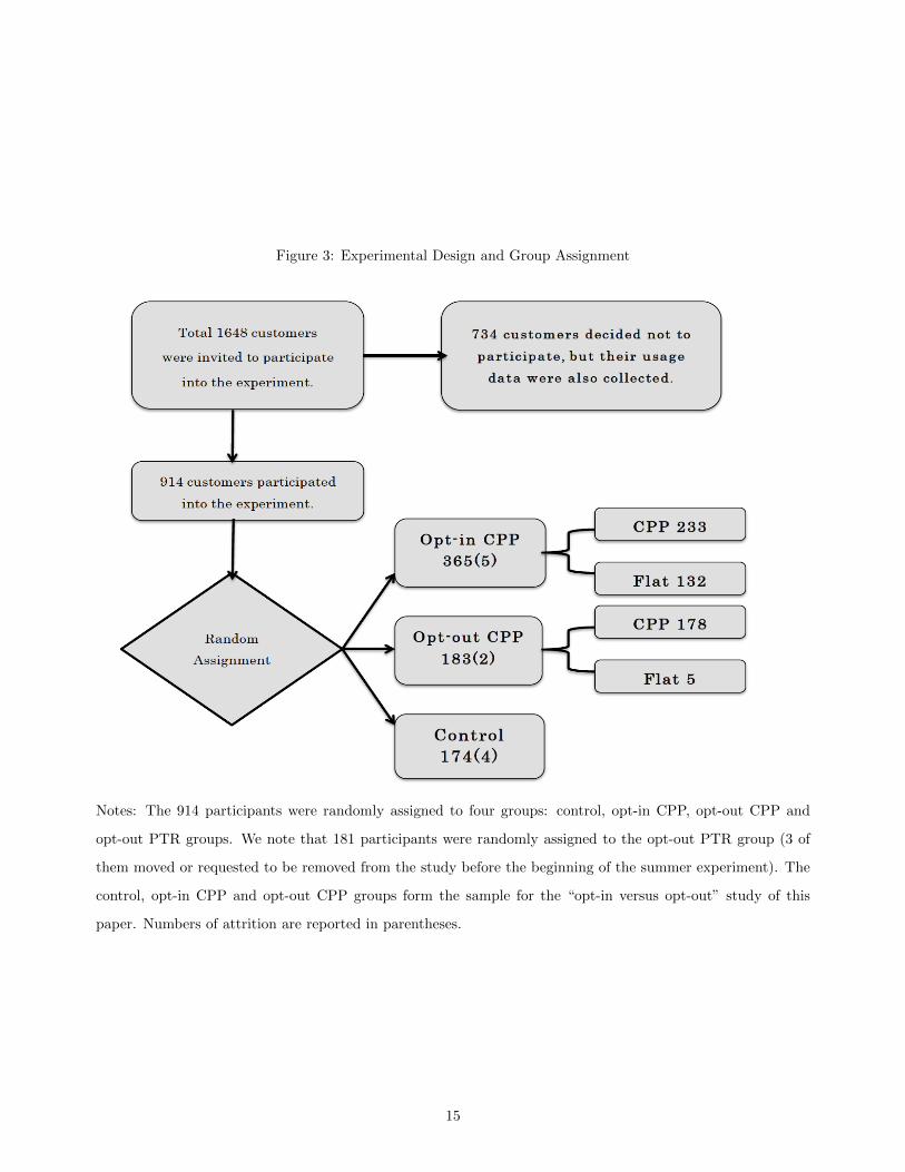
Figure 3: Experimental Design and Group Assignment
Notes: The 914 participants were randomly assigned to four groups: control, opt-in CPP, opt-out CPP and
opt-out PTR groups. We note that 181 participants were randomly assigned to the opt-out PTR group (3 of
them moved or requested to be removed from the study before the beginning of the summer experiment). The
control, opt-in CPP and opt-out CPP groups form the sample for the “opt-in versus opt-out” study of this
paper. Numbers of attrition are reported in parentheses.
15

Table 4: CPP Selection Probit Model of the Opt-in CPP Group
Explanatory Variable (1) (2)
Average Consumption 0.149
(0.182)
On-peak/Off-peak Ratio 0.132*
(0.076)
Observations 365 365
Notes: This table reports the result of the marginal effects for the probit model, in which the dependent variable equals
one if the household assigned to the opt-in CPP treatment group decided to opt into the CPP tariff and zero otherwise.
*, **, and *** show 10%, 5%, and 1% statistical significance, respectively.
1429), we use the consumption data during peak-time period (4 pm to 7 pm) to estimate
the ITTs of the two treatment groups during CPP event hours. Let yit denote household
i’s electricity consumption during a 15-minute interval period t, then our panel data model
controlling for household fixed effects and time fixed effects can be written as:
lnyit =∑
g∈{CPPin,CPPout}
βgITT · I
git + θi + λt + εit (2)
where the indicator variable Igit equals one if household i is in treatment group g with g ∈
{CPPin, CPPout} and if a dynamic pricing event occurs for i in interval t.11 ‘CPPin’ and
‘CPPout’ denote the opt-in CPP group and the opt-out CPP group, respectively. θi denotes a
household fixed effect that controls for persistent differences in consumption across households
and λt denotes a time fixed effect for each 15-minute interval t that accounts for weather and
other shocks specific to t. εit is an unobserved mean zero error term. Here, the explanatory
11We use the natural log of usage for the dependent variable to enable us to interpret the treatment effects approximately
in percentage terms. The treatment effects in the exact percentage terms can be obtained by exp(βgITT ) − 1.
16

variables of interest are the indicators Igit, and the coefficients βgITT correspond to the average
percentage change in electricity usage from assignment to each treatment during pricing events.
Note that high-frequency data on customer-level electricity consumption are likely to be serially
correlated; we, therefore, cluster standard errors at the customer level. Bertrand et al. (2004)
contains a detailed discussion on the consistency of such standard errors in the presence of any
time-dependent correlation pattern in εit within i.
Moreover, as our experiment involves distinct preset default options, which result in very
different customer enrolment rates, we also estimate the TOTs for each treatment group. The
TOT captures the average causal effect of each treatment on the subpopulation of compliers,
that is, households who actually enrolled in the CPP tariff. Although the initial treatment
assignments were implemented randomly in our experiment, some households assigned to the
treatment groups did not enrol in CPP. Thus, the actual receipt of treatment depends on
households’ self-selection and can be regarded as endogenous; in such cases, an ordinary least
squares regression cannot consistently estimate the TOTs. The standard econometric solution
to this problem is to use the instrumental variable (IV) regression. Our TOT specification uses
the initial treatment assignment as an IV for the actual receipt of treatment and is estimated
by using the two-stage least squares regression.12 The randomisation of initial treatment as-
signment and high rates of customer compliance (63.8% for opt-in CPP and 97.2% for opt-out
CPP) ensure both the validity and the strength of the IV in our regressions. The following
specification is used to estimate the TOTs of each treatment group:
lnyit =∑
g∈{CPPin,CPPout}
βgTOT · T
git + θi + λt + εit (3)
where the indicator variable T git equals one if Igit equals one and if household i is actually
enrolled. As with the ITT regressions, we use the on-peak consumption data in the estimation,
and cluster standard errors at the customer level to account for serial correlations in εit.12Our experiment is an RCT with one-sided non-compliance: customers assigned to the treatment groups can decline
the treatment but customers assigned to the control group are not allowed to take the treatment. Therefore, the TOT
in our experiment is equal to the local average treatment effect.
17

3.2 Estimation Results for the Average Treatment Effects
The columns in Table 5 labelled ‘ITT’ report the results from the ITT estimators of each
treatment group. Investigating these results, we find that households in both treatment groups
consumed significantly less electricity during event periods (4 pm to 7 pm on treatment days)
than households in the control group. In particular, both ITTs are statistically different from
zero at the 1% significance level. Despite the fact that many dynamic pricing experiments
have been implemented in hot climates, very few studies have been carried out in moderate
climates.13 It is thus remarkable that significant peak time reduction is achieved in a region
with a rather mild climate (the average maximum temperature of LAC is 77.2◦F during the
summer months) with a low saturation of central air conditioning systems (about 10% in LAC).
More importantly, it turns out that the opt-in CPP group has relatively large estimates of
ITT (9.8% in absolute value). It is remarkable that even with a relatively low enrolment rate,
the opt-in group succeeded in generating a larger aggregate impact than its opt-out counterpart
(5.8%). In addition, the corresponding P-value for the test of difference between the treatment
effects is 0.029. We note the standard economic theory would predict that the opt-out CPP
group generates higher ITTs because it faces a higher (overall) marginal price of electricity than
the opt-in CPP group during on-peak periods and a lower (overall) marginal price during off-
peak periods.14 Moreover, the RCT design ensures that the only systematic difference between
the two treatment groups is the default option, and customers in the two treatment groups
have similar overall potential for on-peak reduction. The ITT result, therefore, suggests that
the opt-in type active enrolment itself had an impact on customers’ subsequent behavior and
made them more responsive during the CPP event periods.
The columns in Table 5 labelled ‘TOT’ report the results for the TOT estimators, that
is, the estimators of the average causal effect on the compliers in each treatment group. Not
surprisingly, the estimated TOT of the opt-in group (14.7%) is much larger than those of the
opt-out group (6.0%). The TOT estimates of the opt-out group are very similar to its ITT
13To the best of our knowledge, Faruqui et al. (2014) is the only existing study in a moderate climate.14During on-peak periods of event days, 97.2% of opt-out CPP customers were on 75 cents/kWh and 2.8% were on
9.52 cents/kWh, while 63.8% of opt-in CPP customers were on 75 cents/kWh and 36.2% were on 9.52 cents/kWh. On
the contrary, during off-peak periods, 97.2% of opt-out CPP customers were on 7.77 cents/kWh and 2.8% were on 9.52
cents/kWh, while 63.8% of opt-in CPP customers were on 7.77 cents/kWh and 36.2% were on 9.52 cents/kWh.
18

Table 5: Average Treatment Effects
Treatment Groups ITT TOT
(1) (2)
CPPin -0.098*** -0.147***
(0.016) (0.025)
CPPout -0.058*** -0.060***
(0.020) (0.021)
P-value[CPPin = CPPout] 0.029** 0.000***
Household Fixed Effect Yes Yes
Time Fixed Effect Yes Yes
Observations 584,616 584,616
Notes: This table reports the estimation results of the average treatment effects of each treatment group during the
dynamic pricing events (4 pm to 7 pm on treatment days). The columns ‘ITT’ and ‘TOT’ show the estimation results
for the intention-to-treat and the treatment-on-the-treated of each treatment group, respectively. Standard errors in
parentheses are clustered at the household level to adjust for serial correlation. *, **, and *** show 10%, 5%, and 1%
statistical significance, respectively.
19

estimates because of the extremely high customer enrolment rates. A potential concern is that
the very high TOTs of the opt-in group are due to customers’ selection into the new tariff: those
who are most price responsive tend to opt in. However, this scenario alone cannot explain the
obtained results because the overall impact (i.e. in terms of the ITT) of the opt-in treatment
is also larger than that of the opt-out treatment. Thus, we expect that the opt-in and opt-out
defaults do have distinct effects on customers’ elasticity.
Table 6 reports estimated average treatment effects for summer and winter separately. The
results for summer are presented in Panel A and those for winter are presented in Panel B,
and they have a similar pattern as those in Table 5. The opt-in CPP group has relatively
large estimates of ITT in absolute value (8.7% for summer and 10.4% for winter), and the
corresponding P-value of the testing of the equality of ITTs is 0.086 for summer and 0.089 for
winter. Not surprisingly, the opt-in TOTs are much larger than the opt-out TOTs in both
summer and winter.
We note that opt-out defaults have been applied successfully in the retirement saving liter-
ature because, in these applications, individuals are not required to take any action after the
initial enrolment. Indeed, opt-out defaults exploit the significant inertia among customers to
obtain extremely high participation in saving plans, and the participants typically retain the
plan contribution rates chosen by companies. However, how do initial defaults affect consumers’
subsequent behaviors has not been well studied in the literature. The situation considered in
this paper is more complicated than the retirement saving, and could be considered to be
two-stage policies as they involve a customer enrolment process in the first stage and (possibly
repeated) treatment interventions in the second stage. Here, the eventual success of the policies
depends not only on initial enrolment rates but also on the attention that could be triggered
by the first-stage procedure, which, in turn, may substantially affect the impact of the second-
stage interventions. In the current context, to face CPP events and achieve significant usage
reductions, households must possess a good understanding of the pricing scheme and incentive
system, identify which home appliances consume a relatively high amount of electricity, and
decide which appliances or services the family is willing to live without during event periods;
all these activities may require considerable attention and cognitive effort.
20
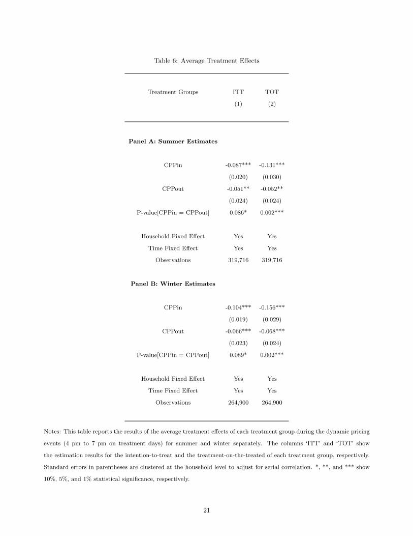
Table 6: Average Treatment Effects
Treatment Groups ITT TOT
(1) (2)
Panel A: Summer Estimates
CPPin -0.087*** -0.131***
(0.020) (0.030)
CPPout -0.051** -0.052**
(0.024) (0.024)
P-value[CPPin = CPPout] 0.086* 0.002***
Household Fixed Effect Yes Yes
Time Fixed Effect Yes Yes
Observations 319,716 319,716
Panel B: Winter Estimates
CPPin -0.104*** -0.156***
(0.019) (0.029)
CPPout -0.066*** -0.068***
(0.023) (0.024)
P-value[CPPin = CPPout] 0.089* 0.002***
Household Fixed Effect Yes Yes
Time Fixed Effect Yes Yes
Observations 264,900 264,900
Notes: This table reports the results of the average treatment effects of each treatment group during the dynamic pricing
events (4 pm to 7 pm on treatment days) for summer and winter separately. The columns ‘ITT’ and ‘TOT’ show
the estimation results for the intention-to-treat and the treatment-on-the-treated of each treatment group, respectively.
Standard errors in parentheses are clustered at the household level to adjust for serial correlation. *, **, and *** show
10%, 5%, and 1% statistical significance, respectively.
21

3.3 Spillover Effects of the Opt-in CPP Group
In general, when the marginal cost of electricity supply is high during on-peak periods, its cost
is also likely to be high during the hours preceding and following these periods. Therefore, if
households simply choose to curtail on-peak consumption and shift their usage into these off-
peak hours (i.e. shoulder hours), the economic benefits of dynamic pricing programmes could
be compromised. For instance, there may be pre-cooling behaviors among CPP households
before summer events, or a ‘backfire’ effect might be observed after summer events when cus-
tomers conduct activities that they avoided during on-peak hours. Similarly, during the winter
experiment, households might have pre-heating behaviors or they might adjust heaters to a
higher temperature as soon as CPP events end.
Interestingly, we find that in our experiment, the opt-in treatment does not result in such
peak–off-peak load shifting and even has spillover effects in the sense that the opt-in CPP
reduction of on-peak electricity usage spills over into the hours preceding and following the
event period. This result is highlighted in Table 7, where we present the estimated average
treatment effects of both treatment groups during the shoulder hours (i.e., the three hours
before the event period and the three hours after the event period). In particular, we use exactly
the same econometric methodology as that used in the previous section for the estimation of
on-peak ITTs in eq.(2) and on-peak TOTs in eq.(3), but with the consumption data preceding
(1 pm to 4 pm) or after (7 pm to 10 pm) the on-peak time window.15
We find that the opt-in CPP group generated a 5.4% usage reduction in terms of the ITT
during the time window before the CPP events and a 4.8% reduction during the time window
after the events, with both coefficients being statistically different from zero at the 1% signif-
icance level. By contrast, we do not find such significant spillover effects for the opt-out CPP
group. Although the coefficients of the opt-out group are also estimated as negative, they are
quite small compared with the estimates of the opt-in group and statistically indistinguishable
from zero. In addition, the tests of the equality of ITTs report P-values of 0.069 and 0.001
for the shoulder hours before and after the CPP events, respectively. Not surprisingly, the
corresponding TOTs of the opt-in group (8.1% before the events and 7.2% after the events) are
15We also estimated using the data from 11 am to 4 pm and from 7 pm to 12 pm, and the results have very similar
patterns.
22

Table 7: Spillover Effects
Treatment Groups ITT TOT ITT TOT
(1) (2) (3) (4)
3 hrs before events 3 hrs after events
CPPin -0.054*** -0.081*** -0.048*** -0.072***
(0.019) (0.028) (0.013) (0.020)
CPPout -0.019 -0.020 -0.003 -0.003
(0.021) (0.022) (0.015) (0.016)
P-value[CPPin = CPPout] 0.069* 0.011** 0.001*** 0.000***
Household Fixed Effect Yes Yes Yes Yes
Time Fixed Effect Yes Yes Yes Yes
Observations 633,539 633,539 584,784 584,784
Notes: This table reports the estimation results of the average treatment effects of each treatment group during the time
window preceding (1 pm to 4 pm) or following (7 pm to 10 pm) the dynamic pricing events. The columns ‘ITT’ and
‘TOT’ show the estimation results for the intention-to-treat and the treatment-on-the-treated for each treatment group
3 hours before the events and 3 hours after the events. Standard errors in parentheses are clustered at the household
level to adjust for serial correlation. *, **, and *** show 10%, 5%, and 1% statistical significance, respectively.
much larger than those of the opt-out group.
In summary, similar to those in the previous section, the results obtained here indicate that
opt-in customers may have been more attentive and responsive than opt-out customers, and
their energy conservation efforts significantly extend beyond peak reduction during CPP event
periods. Such spillover effects may also lead to extra social and environmental benefits.
4 Further Discussion and Concluding Remarks
This paper reports on the result of a randomised field experiment on dynamic pricing pro-
grammes. We find that customers in both opt-in and opt-out programmes significantly reduce
23

their peak electricity consumption. Second, the opt-in group succeeded in generating a larger
aggregate impact (i.e. the ITT) than the opt-out group. Third, we find that only the opt-in
treatment succeeded in triggering significant spillover effects among customers: the opt-in CPP
group generated a usage reduction even during shoulder hours before and after the events.
How large is the net effect of active enrolment on customers’ subsequent behaviors? We
may deduce the lower and upper bounds of its value by using the estimated ITTs and TOTs.
To proceed, let us divide the opt-out CPP participants (97.2% of the opt-out group) into two
types: 1) active customers (around 63.8% of the opt-out group), who would enroll not only
under the opt-out default but also under the opt-in default, and 2) passive customers (around
33.4% (i.e., 97.2% − 63.8%) of the opt-out group), who would only enroll under the opt-out
default.16 Then, the net effect of opt-in enrolment (on active customers) can be written as the
difference between the TOT of active customers in the opt-in group and the TOT of active
customers in the opt-out group (say, TOTCPPin,Active − TOTCPPout,Active), and we can obtain
the bounds on this value by considering several interesting cases. First, its lower bound can be
obtained by considering the case that the passive customers are unresponsive (i.e., have zero
treatment effect) so that the opt-out CPP treatment effect is totally generated by the subgroup
of active customers:
TOTCPPin,Active − TOTCPPout,Active
= TOTCPPin − (ITTCPPout/63.8%)
= −14.7%− (−5.8%/63.8%) = −5.6%,
i.e., 5.6% reduction in electricity usage during CPP events. Second, its upper bound can
be obtained by considering the case that the passive customers are as responsive as the ac-
tive customers (i.e., the two types of customers have the same treatment effect); in this case,
16Note that the random assignment allows the opt-in and opt-out groups to have similar fraction of active and passive
customers.
24

TOTCPPout,Active = TOTCPPout,Passive = TOTCPPout and we obtain:
TOTCPPin,Active − TOTCPPout,Active
= TOTCPPin − TOTCPPout
= −14.7% + 6.0% = −8.7%.
Thus, these calculations suggest that the net effect of opt-in enrolment corresponds to an
average percentage reduction of on-peak usage ranging from 5.6% to 8.7% (i.e., 38% to 59% of
the opt-in TOT) within the subgroup of active customers.
Libertarian paternalists often advocate that policymakers should select the default option
that the majority of people would choose (Thaler and Sunstein, 2003), which typically cor-
responds to opt-out procedures. Our result suggests that the default option chosen by the
majority may not always maximise social efficiency. However, it should not be interpreted as
the evidence that the opt-in default is superior to its opt-out counterpart. Indeed, our focus is
on the effect of default options on consumers’ subsequent behaviors, and we emphasise that the
calculation of an optimal default is not straightforward as it may depend on specific character-
istics of the policy as well as the heterogeneity among customers (e.g., fraction of active and
passive customers); all these factors may vary considerably among different policies. Therefore,
the design of policies with preset defaults should be approached with caution, particularly in
the case of ‘two-stage’ policy interventions. The practical examples of such policies could be
extensive considering that possible second-stage treatments include not only economic incen-
tives but also non-pecuniary behavioral instruments. For instance, Ferraro et al. (2011) and
Ferraro and Price (2013) study three types of non-pecuniary treatments for water conservation:
information dissemination on behavioral and technological modifications, appeal for prosocial
preferences, and provision of social comparisons. Individuals’ attention may also be crucial to
the eventual impact of these treatments.
Finally, an important part of the future research agenda could be the long-run persistency
of the treatment effects generated under different default options. Allcott and Rogers (2014)
show that as the intervention (social comparison by home energy report) is repeated, people
gradually develop new ‘capital stock’ that generates persistent changes in electricity usage.
This capital stock might be physical capital such as energy-efficient light bulbs or appliances or
25

‘consumption capital’ such as a stock of energy use habits in the sense of Becker and Murphy
(1988). In particular, the stock of past conservation behaviors (i.e. rehearsal of conservation
behaviors) is likely to lower the future marginal cost of conservation and, thus, facilitate long-
term habit formation. Here, the active decision-making process triggered by opt-in-type defaults
might positively affect the formation of both physical and consumption capital. For instance,
relatively attentive customers might be more likely to replace their home appliances with energy-
efficient models. Long-term habit formation could also be more likely to occur among these
customers.
Acknowledgements
The authors are grateful for the financial support from the Japan-U.S. Collaborative Smart
Grid Project of the New Energy and Industrial Technology Development Organization. The au-
thors would like to thank Toshiba, Itochu, the Los Alamos Department of Public Utilities, and
the Los Alamos National Laboratory for their enthusiastic support during the implementation
of the experiment. We would also like to thank the participants of the 2014 Workshop on Ex-
perimental Economics at Kyoto University (February 2014), the sixth International Conference
on Integration of Renewable and Distributed Energy Resources (IRDE) in Kyoto (November
2014), the 2015 Annual Conference of the Royal Economic Society at University of Manchester
(March 2015), the fourth Annual Summer Conference of the Association of Environmental and
Resource Economists (AERE) in San Diego (June 2015), the U.S.-Japan Collaborative Smart
Grid Project Workshop in Santa Ana Pueblo (October 2015), and the 12th International Sym-
posium on Econometric Theory and Applications (SETA) at Waikato University (February
2016).
26

References
Abadie, A., and S. Gay (2006): “The impact of presumed consent legislation on cadaveric organ donation: A cross-
country study,” Journal of Health Economics, 25(4), 599–620.
Allcott, H., and T. Rogers (2014): “The short-run and long-run effects of behavioral interventions: Experimental
evidence from energy conservation,” American Economic Review, 104(10), 3003–3037.
Becker, G. S., and K. M. Murphy (1988): “A theory of rational addiction,” Journal of political Economy, 96(4),
675–700.
Bertrand, M., E. Duflo, and S. Mullainathan (2004): “How much should we trust differences-in-differences
estimates?,” The Quarterly Journal of Economics, 119(1), 249–275.
Borenstein, S. (2013): “Effective and equitable adoption of opt-in residential dynamic electricity pricing,” Review of
Industrial Organization, 42(2), 127–160.
Chapman, G. B., M. Li, H. Colby, and H. Yoon (2010): “Opting in vs opting out of influenza vaccination,” Journal
of the American Medical Association, 304(1), 43–44.
Chetty, R., J. N. Friedman, S. Leth-Petersen, T. H. Nielsen, and T. Olsen (2014): “Active vs. passive decisions
and crowd-out in retirement savings accounts: Evidence from Denmark,” The Quarterly Journal of Economics, 129(3),
1141–1219.
Choi, J. J., D. Laibson, B. C. Madrian, and A. Metrick (2002): “Defined contribution pensions: Plan rules,
participant choices, and the path of least resistance,” in Tax Policy and the Economy, Volume 16, pp. 67–114. MIT
Press.
DellaVigna, S., and U. Malmendier (2006): “Paying not to go to the gym,” The American Economic Review, 96(3),
694–719.
Faruqui, A., and S. Sergici (2011): “Dynamic pricing of electricity in the mid-Atlantic region: Econometric results
from the Baltimore gas and electric company experiment,” Journal of Regulatory Economics, 40(1), 82–109.
Faruqui, A., S. Sergici, and L. Akaba (2014): “The impact of dynamic pricing on residential and small commercial
and industrial usage: New experimental evidence from Connecticut,” The Energy Journal, 35(1), 137–160.
Ferraro, P. J., J. J. Miranda, and M. K. Price (2011): “The persistence of treatment effects with norm-based
policy instruments: evidence from a randomized environmental policy experiment,” The American Economic Review,
101(3), 318–322.
Ferraro, P. J., and M. K. Price (2013): “Using nonpecuniary strategies to influence behavior: Evidence from a
large-scale field experiment,” Review of Economics and Statistics, 95(1), 64–73.
Fowlie, M., C. Wolfram, C. A. Spurlock, A. Todd, P. Baylis, and P. Cappers (2017): “Default effects and
follow-on behavior: Evidence from an electricity pricing program,” Discussion Paper WP280, Energy Institute at Haas
School of Business, UC Berkeley.
Ito, K., T. Ida, and M. Tanaka (2017): “Moral Suasion and Economic Incentives: Field Experimental Evidence from
Energy Demand,” American Economic Journal: Economic Policy, Forthcoming.
27

Jessoe, K., and D. Rapson (2014): “Knowledge is (less) power: Experimental evidence from residential energy use,”
The American Economic Review, 104(4), 1417–1438.
Johnson, E. J., and D. Goldstein (2003): “Do defaults save lives?,” Science, 302(5649), 1338–1339.
Johnson, E. J., and D. G. Goldstein (2013): “Decisions by default,” Behavioral Foundations of Policy, e.d. by
E.SHAFIR, Princeton University Press, Princeton, pp. 417–427.
Johnson, E. J., J. Hershey, J. Meszaros, and H. Kunreuther (1993): “Framing, probability Distortions, and
insurance Decisions,” Journal of Risk and Uncertainty, 7(1), 35–51.
Madrian, B. C., and D. F. Shea (2001): “The power of suggestion: inertia in 401 (k) participation and savings
behavior,” The Quarterly Journal of Economics, 116(4), 1149–1187.
Potter, J., S. George, and L. Jimenez (2014): “SmartPricing options final evaluation: The final report on pilot
design, implementation, and evaluation of the Sacramento Municipal Utility District’s consumer behavior study,”
Sacramento Municipal Utility District.
Spital, A. (1995): “Mandated choice: a plan to increase public commitment to organ donation,” Journal of the American
Medical Association, 273(6), 504–506.
Thaler, R. H., and S. Benartzi (2004): “Save more tomorrow?: Using behavioral economics to increase employee
saving,” Journal of political Economy, 112(S1), S164–S187.
Thaler, R. H., and C. R. Sunstein (2003): “Libertarian paternalism,” American Economic Review, 93(2), 175–179.
Wolak, F. A. (2006): “Residential customer response to real-time pricing: The Anaheim critical peak pricing experi-
ment,” Center for the Study of Energy Markets.
(2010): “An experimental comparison of critical peak and hourly pricing: the PowerCentsDC program,” De-
partment of Economics, Stanford University.
(2011): “Do residential customers respond to hourly prices? Evidence from a dynamic pricing experiment,” The
American Economic Review, 101(3), 83–87.
28

A Online Appendix A (Not for Publication)
A.1 High-frequency Treatment Effects
The estimation results in Sections 3.2 and 3.3 in the paper demonstrate that, on average, the
opt-in treatment has a relatively large impact of consumption reduction during both the CPP
event period and the time window preceding and following CPP events. However, a potential
concern is that although the overall impact of the opt-in CPP group is relatively large, the
opt-in treatment effect might have considerable variation and could be larger than the opt-out
treatment effect during some parts of the event period but smaller during other parts.
In this section, we study this issue by making use of our high-frequency data. Specifically, we
estimate the ITTs and TOTs for each 15-minute time interval during both event and shoulder
hours (i.e. 1 pm to 10 pm on treatment days), using a one-hour rolling window to smooth over
idiosyncratic variation. For each time index d, we use observations that are 15 or 30 minutes
before d, observations on time d, and observations 15 or 30 minutes after d; the panel fixed
effects regression for the corresponding ITTs can thus be written as
lnyit =∑
g∈{CPPin,CPPout}
βgITT · I
git + θi + λt + εit, ∀t ∈ {d− 30, d− 15, d, d+ 15, d+ 30} (1)
The corresponding TOTs are estimated using the indicator variable Igit as an IV.
Figure A1 plots the estimation results of summer high-frequency ITT/TOTs and the cor-
responding (pointwise) 95% confidence intervals; several important features emerge from the
figure. First, it is reassuring to find that the estimated values of the opt-in treatment effects
are relatively large throughout the whole estimation period. Second, we observe from the fig-
ure that the consumption reduction of both groups gradually increases as CPP events begin,
reaches its peak around 5 pm to 6 pm, and gradually backslides afterwards. Third, the treat-
ment effects of the opt-out CPP group seem to be particularly weak during the beginning part
of the event period (4 pm to 5 pm). By contrast, opt-in ITTs remain higher than 7% during
this time window; such stability in treatment effects may be important from utility compa-
nies’ or policymakers’ perspectives because they can be confident that during any period of the
event, a certain level of on-peak usage reduction is expected. Figure A2 plots the results for
1

the winter season, showing that the pattern of these treatment effects is similar to that found
in the summer sample, with the opt-in treatment effects being relatively large throughout the
whole time window. We also observe that the opt-out ITT/TOT estimates (and corresponding
confidence intervals) become slightly positive during some periods of time after the CPP events,
indicating that some opt-out customers may have offset the conservation during event hours by
increasing usage in adjacent non-event hours. As we discussed at the beginning of Section 3.3,
such peak–off-peak load shifting might compromise the overall impact of the intervention.
A.2 Heterogeneous Treatment Effects
In this section, we explore the possible variation of treatment effects across our participants
and attempt to gain further understanding on the mechanisms through which the two treat-
ments affect customer behaviours. Our investigation proceeds by analysing the behaviour of
households that have electric appliances such as ACs (including centralised and window ACs)
and electric heaters. These appliances account for a large proportion of household electricity
usage and are more likely to be related to the level of households’ willingness or motivation to
reduce on-peak consumption compared with other home appliances. Suppose that on a certain
summer treatment day, the weather is very hot. If some households’ conservation motivation
is relatively low, the high temperature may have a negative impact on the willingness of these
customers to reduce electricity consumption by adjusting their ACs. Then, we should be able
to observe a decrease in the treatment effect among AC holders, particularly among AC holders
in the less motivated treatment group. Similar arguments could be made for electric heater
owners during the winter experiment because cold weather may have a negative impact on
the willingness of customers, particularly less motivated customers, to reduce consumption by
adjusting their heaters.
By using the summer analysis for example, we estimate the following panel fixed effects
2

Figure A1: Summer High-Frequency Treatment Effects−
.2−
.15
−.1
−.0
50
.05
Tre
atm
en
t E
ffe
ct
(Pe
rce
nta
ge
)
14 15 16 17 18 19 20 21Hour of day
CPPin ITT CPPin ITT 95%CI
CPPout ITT CPPout ITT 95%CI
(a) ITT
−.2
−.1
5−
.1−
.05
0.0
5
14 15 16 17 18 19 20 21Hour of day
CPPin TOT CPPin TOT 95%CI
CPPout TOT CPPout TOT 95%CI
(b) TOT
Figure A2: Winter High-Frequency Treatment Effects
−.2
−.1
5−
.1−
.05
0.0
5T
rea
tme
nt
Eff
ect
(Pe
rce
nta
ge
)
14 15 16 17 18 19 20 21Hour of day
CPPin ITT CPPin ITT 95%CI
CPPout ITT CPPout ITT 95%CI
(a) ITT
−.2
−.1
5−
.1−
.05
0.0
5
14 15 16 17 18 19 20 21Hour of day
CPPin TOT CPPin TOT 95%CI
CPPout TOT CPPout TOT 95%CI
(b) TOT
3

model augmented with interaction terms:
lnyit =∑
g∈{CPPin,CPPout}
βg1 · I
git +
∑g∈{CPPin,CPPout}
βg2 · I
git · I[i,Cooler]
+∑
g∈{CPPin,CPPout}
βg3 · I
git · I[t,HotEventDay] +
∑g∈{CPPin,CPPout}
βg4 · I
git · I[i,Cooler] · I[t,HotEventDay]
+ θi + λt + εit
(2)
where Igit has the same definition as in Section 3 of the paper. Additionally, we introduce two
indicator variables I[i,Cooler] and I[t,HotEventDay] for the current analysis. Specifically, I[i,Cooler]
equals one if household i owns ACs and zero otherwise, while I[t,HotEventDay] equals one if
the time interval t is during a treatment day whose temperature is higher than the average
temperature of the 14 summer treatment days. Therefore, in this interaction model, βg1 captures
the (conditional) average treatment effect for group g households without ACs on relatively
cool treatment days whose temperatures are below the 14-treatment-day average (i.e. the case
that I[i,Cooler] = 0 and I[t,HotEventDay] = 0); similarly, βg1 + βg
2 corresponds to the case that
I[i,Cooler] = 1 and I[t,HotEventDay] = 0, and βg1 +βg
3 corresponds to the case that I[i,Cooler] = 0 and
I[t,HotEventDay] = 1. Finally, βg1 + βg
2 + βg3 + βg
4 captures the treatment effect for AC holders on
relatively hot treatment days (i.e. I[i,Cooler] = 1 and I[t,HotEventDay] = 1). For the purpose of the
current analysis, we are particularly interested in the estimates of βg4 because these capture the
interaction effect between ACs and temperatures on treatment days. Similarly, we can specify
the econometric model for the winter analysis as follows:
lnyit =∑
g∈{CPPin,CPPout}
βg1 · I
git +
∑g∈{CPPin,CPPout}
βg2 · I
git · I[i,Heater]
+∑
g∈{CPPin,CPPout}
βg3 · I
git · I[t,ColdEventDay] +
∑g∈{CPPin,CPPout}
βg4 · I
git · I[i,Heater] · I[t,ColdEventDay]
+ θi + λt + εit
(3)
where we introduce indicator variables I[i,Heater] and I[t,ColdEventDay]; I[i,Heater] equals one if
household i owns electric heaters, while I[t,ColdEventDay] equals one if time interval t is during
a treatment day with a temperature lower than the average temperature of the 15 winter
4

treatment days.
The summer estimation results are presented in Table A1. The estimates of βCPPin1 and
βCPPout1 are −7.8% and −5.0%, respectively. In addition, all the signs of βCPPin
2 , βCPPout2 ,
βCPPin3 , and βCPPout
3 are negative, indicating that the treatment effects might have a tendency
to become slightly larger when households have ACs or when the event day temperature is rel-
atively high; all these coefficients are too small to be statistically significant. Finally, and most
interestingly, we find that both βCPPin4 (3.9%) and βCPPout
4 (5.8%) are positive, with βCPPout4 be-
ing relatively large and statistically significant. Therefore, the estimates of βCPPin4 and βCPPout
4
suggest that AC holders, particularly those in the opt-out CPP group, may have generated
relatively small on-peak reduction during hot treatment days. This result is consistent with
our hypothesis that opt-out households could be less motivated than opt-in households. The
winter results are presented in Table A2; the patterns of the estimates of βCPPin4 and βCPPout
4
are similar to those in the summer results, although βCPPout4 is not statistically significant.
A.3 Analysis of Participant Characteristics
The usage data of both participants and non-participants allow us to investigate the type
of customer likely to participate in our dynamic pricing programme. Here, we assume that
individual decisions on whether to participate in the experiment depend on a linear function of
customer-specific characteristic variables Xi:
Yi = 1 (X ′iδ + vi ≥ 0) (4)
where Yi equals one if household i decides to participate in the experiment and zero otherwise.
Assuming that vi is normally distributed, this can be estimated using a probit regression.
We construct household-level average usage and the average on-peak/off-peak ratio of usage
as the customer characteristic variables using pre-event consumption data. Table A3 reports
the estimation result of the probit regression. The estimated coefficient on average usage is
positive and statistically significant at the 1% level, while the on-peak/off-peak ratio estimate
is insignificant.
5

Table A1: Heterogeneous Treatment Effects (Cooler)
(1)
CPPin -0.078***(0.023)
CPPout -0.050*(0.027)
CPPin × 1[Cooler] -0.029(0.029)
CPPout × 1[Cooler] -0.016(0.046)
CPPin × 1[Hot Event Day] -0.010(0.023)
CPPout × 1[Hot Event Day] -0.006(0.025)
CPPin × 1[Cooler] × 1[Hot Event Day] +0.039(0.029)
CPPout × 1[Cooler] × 1[Hot Event Day] +0.058*(0.030)
Household Fixed Effect YesTime Fixed Effect Yes
Observations 278,391
Notes: This table reports the results of summer heterogeneous treatment effects. Standard errors in parenthesesare clustered at the household level to adjust for serial correlation. *, **, and *** show 10%, 5%, and 1%statistical significance, respectively.
6

Table A2: Heterogeneous Treatment Effects (Heater)
(1)
CPPin -0.114***(0.033)
CPPout -0.075**(0.032)
CPPin × 1[Heater] +0.011(0.033)
CPPout × 1[Heater] +0.007(0.041)
CPPin × 1[Cold Event Day] -0.020(0.026)
CPPout × 1[Cold Event Day] -0.014(0.031)
CPPin × 1[Heater] × 1[Cold Event Day] +0.010(0.024)
CPPout × 1[Heater] × 1[Cold Event Day] +0.036(0.031)
Household Fixed Effect YesTime Fixed Effect Yes
Observations 220,272
Notes: This table reports the results of winter heterogeneous treatment effects. Standard errors in parenthesesare clustered at the household level to adjust for serial correlation. *, **, and *** show 10%, 5%, and 1%statistical significance, respectively.
Table A3: Selection Probit Model of Participants
Explanatory Variable (1) (2)
Average Consumption 0.474***(0.091)
On-peak/Off-peak Ratio -0.036(0.026)
Observations 1634 1634
Notes: This table reports the result of the estimated marginal effects for the probit model, in which thedependent variable equals one if the household decided to participate in the experiment and zero otherwise. *,**, and *** show 10%, 5%, and 1% statistical significance, respectively.
7
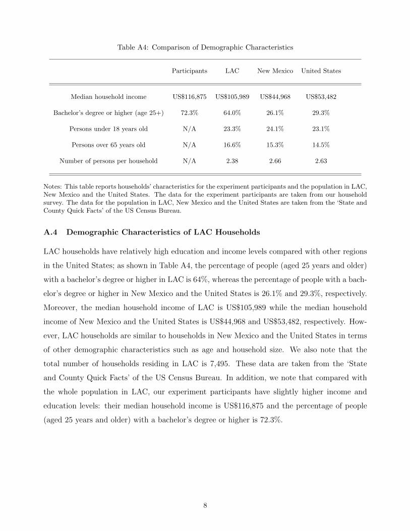
Table A4: Comparison of Demographic Characteristics
Participants LAC New Mexico United States
Median household income US$116,875 US$105,989 US$44,968 US$53,482
Bachelor’s degree or higher (age 25+) 72.3% 64.0% 26.1% 29.3%
Persons under 18 years old N/A 23.3% 24.1% 23.1%
Persons over 65 years old N/A 16.6% 15.3% 14.5%
Number of persons per household N/A 2.38 2.66 2.63
Notes: This table reports households’ characteristics for the experiment participants and the population in LAC,New Mexico and the United States. The data for the experiment participants are taken from our householdsurvey. The data for the population in LAC, New Mexico and the United States are taken from the ‘State andCounty Quick Facts’ of the US Census Bureau.
A.4 Demographic Characteristics of LAC Households
LAC households have relatively high education and income levels compared with other regions
in the United States; as shown in Table A4, the percentage of people (aged 25 years and older)
with a bachelor’s degree or higher in LAC is 64%, whereas the percentage of people with a bach-
elor’s degree or higher in New Mexico and the United States is 26.1% and 29.3%, respectively.
Moreover, the median household income of LAC is US$105,989 while the median household
income of New Mexico and the United States is US$44,968 and US$53,482, respectively. How-
ever, LAC households are similar to households in New Mexico and the United States in terms
of other demographic characteristics such as age and household size. We also note that the
total number of households residing in LAC is 7,495. These data are taken from the ‘State
and County Quick Facts’ of the US Census Bureau. In addition, we note that compared with
the whole population in LAC, our experiment participants have slightly higher income and
education levels: their median household income is US$116,875 and the percentage of people
(aged 25 years and older) with a bachelor’s degree or higher is 72.3%.
8