Czech Technical University in Prague

Faculty of Nuclear Science and Physical Engineering

BACHELOR´S THESIS

Lucie Strmiskova

Supervisor: Dr. Ing. Pavel Soldan

July 21, 2007

Acknowledgements

I would like to thank Dr. Ing. Pavel Soldan for his support, valueable consultationsand careful corrections.

Nazev prace:

Chaoticky oscilator

Autor: Lucie Strmiskova

Obor: Matematicke inzenyrstvı

Zamerenı: Matematicka fyzika

Druh prace: Bakalarska prace

Vedoucı prace: Dr. Ing. Pavel Soldan, Katedra fyziky, Fakulta jaderna a fyzikalne inzenyrska,

Ceske vysoke ucenı technicke v Praze

Abstrakt: Uvedeme definice stability a shrneme dulezite vlastnosti resenı prevazne linearnıch

diferencialnıch rovnic. Seznamıme se s jejich vyuzitım pro urcenı stability resenı rovnic ne-

linearnıch. Popıseme nejbeznejsı bifurkace, ktere nastavajı pro jednoparametricky system.

Zıskane znalosti uplatnıme pri rozboru chovanı dvou jednoduchych elektrickych obvodu.

Klıcova slova: stacionarnı body, orbity, stabilita, Hurwitzovo kriterium, bifurkace

Title:

Chaotic oscillator

Author: Lucie Strmiskova

Abstract: We present the stability definitions and we summarize the important solution

properties of mainly linear differential equations. We use gained knowledge for deter-

mining the stability of nonlinear differential equations. We describe the most common

bifurcations in systems with one parameter. We apply the previous by investigating the

behaviour of two simple electrical circuits.

Key words: stationary points, periodic orbits, Hurwitz´s criterion, stability, bifurcations

Contents

Introduction 2

1 Differential equations and stability of their solutions 31.1 Differential equations . . . . . . . . . . . . . . . . . . . . . . . . . . . 31.2 Stability . . . . . . . . . . . . . . . . . . . . . . . . . . . . . . . . . . 41.3 Linear stability . . . . . . . . . . . . . . . . . . . . . . . . . . . . . . 71.4 Linearization of nonlinear systems . . . . . . . . . . . . . . . . . . . . 17

2 Bifurcations 222.1 Transcritical bifurcation . . . . . . . . . . . . . . . . . . . . . . . . . 222.2 Saddle-node bifurcation . . . . . . . . . . . . . . . . . . . . . . . . . . 242.3 Pitchfork bifurcation . . . . . . . . . . . . . . . . . . . . . . . . . . . 242.4 Hopf bifurcation . . . . . . . . . . . . . . . . . . . . . . . . . . . . . . 262.5 Classification of the stationary points . . . . . . . . . . . . . . . . . . 28

2.5.1 One-dimensional case . . . . . . . . . . . . . . . . . . . . . . . 282.5.2 Two-dimensional case . . . . . . . . . . . . . . . . . . . . . . . 302.5.3 Three-dimensional case . . . . . . . . . . . . . . . . . . . . . . 32

3 Chaotic oscillators 353.1 Vilnius oscillator . . . . . . . . . . . . . . . . . . . . . . . . . . . . . 363.2 Chaos generator . . . . . . . . . . . . . . . . . . . . . . . . . . . . . . 38

1

Introduction

Chaos is a term used for an erratic, almost random, behaviour of time-dependentdynamical systems, which we otherwise consider to be simple and expectable.

Roots of the chaos theory date back to the beginning of the twentieth century,when Henri Poincare, while working on the three-body problem, discovered thatthere can exist orbits that are aperiodic and that are not still increasing nor ap-proaching to a fixed point.

In the sixties, when it became evident, that the linear theory was not able toexplain most of the observed phenomena, the nonlinear theory progressed morerapidly. Stimulating factor had been, of course, the birth of efficient computers.

In 1960, the American meteorologist Edward Lorenz was concerned by the prob-lem of weather predictions. He set up twelve differential equations to model aclimate. He noted the results gained by numerical simulation, and one year later,he tried to repeat these calculations. To his large surprise, the results were totallydifferent. He noticed that in the first calculation he inserted the number 0,506127but then he used rounded off value 0,506. Thus he discovered that nonlinear equa-tions are very sensitive to initial conditions. This sensitivity is popularly called thebutterfly effect (Lorenz summarized his results in a lecture with a name: ”Does aflap of butterfly wings in Brazil set off a tornado in Texas?”)

Presently, the chaos theory is a very popular research topic and it is not limitedonly to meteorology or physics. In biology for example, it is used for modeling thepopulation growth or brain behaviour by an epileptic fit. Chaotic behaviour alsooccurs in some chemical reactions. Some mathematicians try to explain the moveof shares at exchange using the chaos theory. In this bachelor´s thesis, we will bedeal with chaotic circuits.

2

Chapter 1

Differential equations and stabilityof their solutions

1.1 Differential equations

We summarize some important properties of differential equations in this section.Consider a system of the first order differential equations in its standard form:

x1 = f1(x1, . . . , xn)

...

xn = fn(x1, . . . , xn),

where fi are real functions defined in some domain G ⊆ Rn, xi are real variables

and the dot denotes the differentiation with respect to time. The system is oftenwritten in a vector form:

~x = f(~x), ~x ∈ Rn. (1.1)

Such equations, where time does not appear explicitly on the right hand side of theequations, are called autonomous. On the other hand, the term non-autonomous

denotes the equations where time does appear explicitly. In this bachelor’s thesis,we will focus mainly on the autonomous systems.

Definition 1. Vector function ~x(t) is a solution of the equation (1.1) in an openinterval I iff:1. the differentiation ~x exists and it is continuous in I2. ~x(t) ∈ G ∀t ∈ I

3. ~x(t) = f(~x(t)) ∀t ∈ I.

Now we would like to know when the differential equation is soluble. The followingtheorem gives us the answer.

3

Theorem 1 (Local existence and uniqueness of the solution). Suppose ~x =f(~x) and f : R

n → Rn is continuously differentiable. Then there exist maximal

t1 > 0 and t2 > 0 such that a solution ~x(t) with initial condition ~x(t0) = ~x0 existsand is unique for all t ∈ (t0 − t1, t0 + t2).

The proof of this theorem can be found in almost all textbooks on differentialequations (e.g. [2]) a we will not give it here.

We can imagine the solution of differential equation (1.1) with initial condition~x(0) = ~x0 as a point of an n-dimensional space called the phase space. The valueof ~x(t) represents the state of the dynamical system described by the differentialequation at given time t, so the phase space is a set of all possible states of thesystem in this sense. The vector ~x(t) traces out a curve in R

n. This curve is oftencalled an integral curve, orbit or trajectory through x0. It will be signed as x(x0, t)in the following pages whether x is one-dimensional or not.

Several significant trajectories exist in the phase space. For us, stationary pointsand periodic orbits are the most important.

Definition 2. A point x0 is called a stationary (fixed or equlibrium) point iff itdoes not change during the time evolution, i.e.:

d

dtx(x0, t) = 0 ⇔ x(x0, t) = x0 ∀t ≥ 0.

Definition 3. A point x0 is periodic with period T (T > 0) iff

x(x0, t+ T ) = x(x0, t) ∀t ∈ R and x(x0, t+ s) 6= x(x0, t) ∀s ∈ (0, T ).

Closed curve Γ = y ∈ Rn|y = x(x0, t), 0 ≤ t ≤ T is called a periodic orbit.

1.2 Stability

The problem of the solution stability of differential equations has been mentionedin the introduction. In this paragraph, we would like to analyze this problem in amore detail. We chose the most commonly used definitions of stability from about60 different definitions and we will concentrate on them.

Definition 4. A point x0 is Liapounov stable iff

(∀ǫ > 0)(∃δ > 0)(∀y0 ∈ Rn)(|x0 − y0| < δ ⇒ |x(x0, t) − y(y0, t)| < ǫ ∀t ≥ 0).

It means that the distance of two trajectories, which start nearby, does not breakcertain bound during the time evolution. By the sign |.| is meant the norm in R

n.All norms are equivalent in R

n so we will choose the most convenient norm forconcrete examples.

4

Definition 5. A point x0 is quasi-asymptotically stable iff

(∃δ > 0)(∀y0 ∈ Rn)(|x0 − y0| < δ ⇒ |x(x0, t) − y(y0, t)| → 0 as t→ ∞).

It means that all nearby trajectories will approach the trajectory x(x0, t) throughx0. However, we should realize that this definition only says what happens whentime tends to infinity so the orbits do not have to tend to each other at finite time.

The following two simple examples illustrate the fact that the Liapounov stabilitydoes not results from quasi-asymptotical stability and vice versa.

Example 1. Consider the system

x1 = −x2 x2 = x1

with solutionx1 = r0.cos(t+ ϕ) x2 = r0.sin(t+ ϕ).

Take two nearby points:

x = r0.(cos(t+ ϕ), sin(t+ ϕ)) y = (r0 + δ).(cos(t+ ϕ), sin(t+ ϕ))

|x− y| = |δ.(cos(t+ ϕ), sin(t+ ϕ))| = δ

The solutions are concentric circles about the origin. The distance between twonearby points remains constant so all points are Liapounov stable but none arequasi-asymptotically stable. ♠

Example 2. Take the non-autonomous system

x1 =x1

t− t2x1x2

2 x2 = −x2

t

with solution

x1(t) = x01t

t0e−(x02t0)2(t−t0) x2(t) = x02

t0

t∀t ≥ t0 > 0.

We show that the stationary point x = 0 is quasi-asymptotically stable although itis not Liapounov stable. The definitions used for the stability of non-autonomoussystems slightly differ from the ones for autonomous systems but the difference isnot important for this purpose.

It is obvious that limt→∞|x(t)| = 0 ∀t0, x0 so the condition for quasi-asymptoticalstability is fulfilled.

Take ǫ = 1e, t0 = 1, x01 = δ2, x02 = δ, ∀δ > 0.

x1(t) = δ2te−δ2(t−1), x2(t) =δ

tt ≥ 1

5

In special time t1 = 1 + 1δ2 , the solution looks:

x1(t1) = δ2

(

1 +1

δ2

)

e−1 =δ2 + 1

e>

1

e= ǫ

x2(t) =δ3

δ2 + 1

|x(t1)| = |x1(t1)| + |x2(t2)| > ǫ

♠

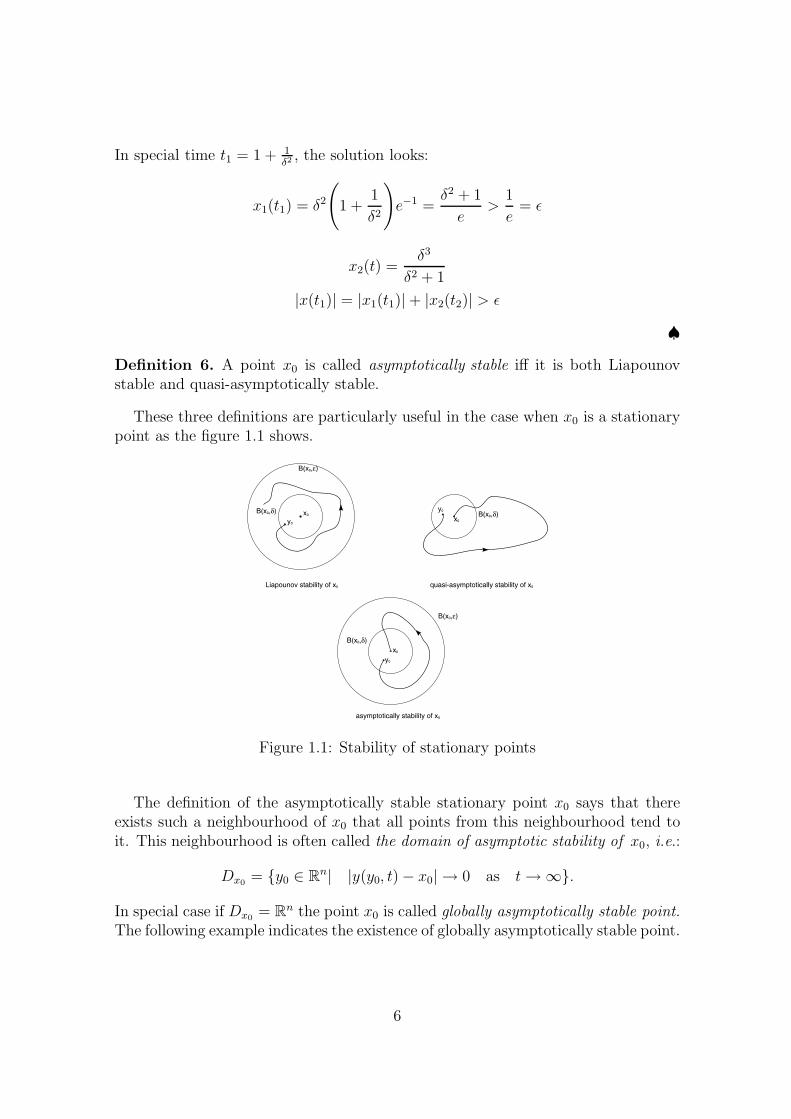
Definition 6. A point x0 is called asymptotically stable iff it is both Liapounovstable and quasi-asymptotically stable.

These three definitions are particularly useful in the case when x0 is a stationarypoint as the figure 1.1 shows.

Figure 1.1: Stability of stationary points

The definition of the asymptotically stable stationary point x0 says that thereexists such a neighbourhood of x0 that all points from this neighbourhood tend toit. This neighbourhood is often called the domain of asymptotic stability of x0, i.e.:

Dx0= y0 ∈ R

n| |y(y0, t) − x0| → 0 as t→ ∞.

In special case if Dx0= R

n the point x0 is called globally asymptotically stable point.

The following example indicates the existence of globally asymptotically stable point.

6

Example 3. Take the system x1 = −x2 x2 = 2x1 − 3x2 with solution

x(x0, t) = ((2x01 − x02).e−t + (x02 − x01).e

−2t, (2x01 − x02).e−t + 2(x02 − x01).e

−2t).

It is obvious that the stationary point y0 = 0 is globally asymptotically stablebecause all trajectories with any initial condition x0 approach it. ♠

Example 4. Consider the system r = 0 θ = 1 + r with solution

r(t) = r0 θ(t) = (1 + r0)t+ θ0.

This example is very similar to example 1. The solutions also lie on concentriccircles around the origin and we expect that all points are Liapounov stable too.However the origin is the only point that fulfills the previous definition.

Take two nearby points (r0, 0) and (r0 + δ, 0) and find phase lag

∆θ = (1 + r0)t− (1 + r0 + δ)t = −δt.

It is apparent that the distance of such chosen points is grater then 2r0 in some spe-cial times although the orbits as a whole remain nearby. We see that the definitionused for points cannot be the most suitable for periodic orbits. For this reason wetry to find another stability definition more convenient for closed orbits. ♠

Let Γ = y ∈ Rn|y = x(x0, t), 0 ≤ t ≤ T. We define the neighbourhood N(Γ, ǫ)

as follows:N(Γ, ǫ) = x ∈ R

n|∃y ∈ Γ : |x− y| < ǫ.

Definition 7. A periodic orbit Γ is orbital stable iff

(∀ǫ > 0)(∃δ > 0)(x0 ∈ N(Γ, ǫ) ⇒ x(x0, t) ∈ N(Γ, ǫ) ∀t ≥ 0).

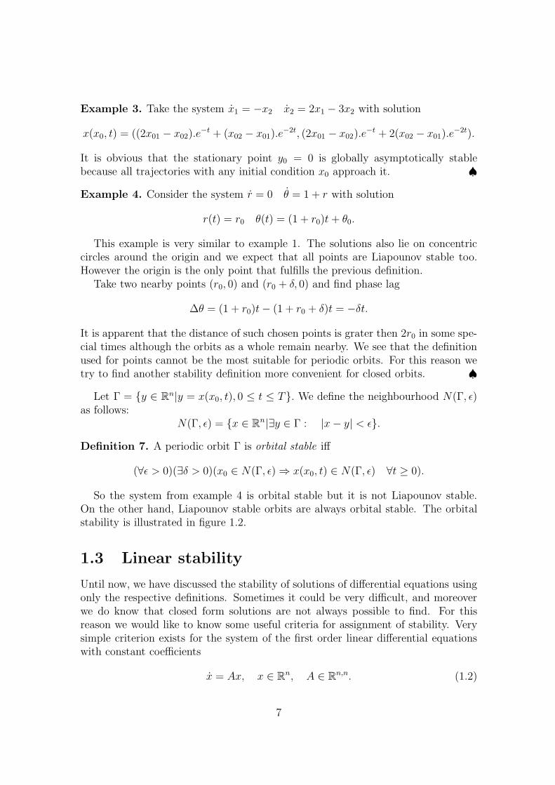
So the system from example 4 is orbital stable but it is not Liapounov stable.On the other hand, Liapounov stable orbits are always orbital stable. The orbitalstability is illustrated in figure 1.2.

1.3 Linear stability

Until now, we have discussed the stability of solutions of differential equations usingonly the respective definitions. Sometimes it could be very difficult, and moreoverwe do know that closed form solutions are not always possible to find. For thisreason we would like to know some useful criteria for assignment of stability. Verysimple criterion exists for the system of the first order linear differential equationswith constant coefficients

x = Ax, x ∈ Rn, A ∈ R

n,n. (1.2)

7

Figure 1.2: Orbital stability

We summarize the most important properties of the system (1.2) briefly at first.More detailed information could be found in [2].

1. The matrix A has n distinct eigenvalues λ1, . . . , λn with respective eigenvectorsh(1), . . . , h(n). Then the vector functions h(1)eλ1t, . . . , h(n)eλnt form the fundamentalsystem of solutions of (1.2).

2. The matrix A has m distinct eigenvalues λ1, . . . , λm, m < n. Denote the mul-tiplicity of λi as a root of characteristic multinominal of the matrix A as li and thenumber of linearly independent eigenvectors respective to λi as pi. We know thatpi ≤ li so

∑ni=1 pi ≤

∑ni=1 li = n. Therefore we do not suffice with eigenvectors to

form the fundamental system.We transfer the matrix A to its Jordan normal form Q = H−1AH, detH 6= 0 to

solve the system x = Ax. Let us take x = Hy. Then x = Ax⇔ y = Qy.

Denote the identity matrix of the order k as Ik, the null matrix as O and supposethat the matrix of the order k, Pk, has the following form:

Pk =

0 1 0 0 . . . 00 0 1 0 . . . 0...0 0 0 0 . . . 10 0 0 0 . . . 0

So the Jordan normal form of the matrix A can be written as a block diagonalmatrix:

Q =

λ1Ik1+ Pk1

O O . . . O

O λ2Ik2+ Pk2

O . . . O...O O O . . . λrIkr

+ Pkr

.

8

The number of diagonal blocks r is determined by the condition r =∑m

i=1 pi ≥ m.For this reason the eigenvalues λ1, . . . , λr do not have to be distinct. The size ofblocks will be determined later.

We may imagine the system y = Qy as r independent subsystems and solve themseparately. The fundamental matrix of each subsystem is then:

Uλiki(t) =

1 t t2

2!. . . tki−1

(ki−1)!

0 1 t . . . tki−2

(ki−2)!...0 0 0 . . . 1

eλit. (1.3)

Hence the fundamental matrix U(t) of system y = Qy is a block diagonal matrixwith blocks (1.3).

U(t) =

Uλ1k1(t) O . . . O

O Uλ2k2(t) . . . O

...O . . . O Uλrkr

(t)

(1.4)

It is obvious that the matrixHU(t) is a fundamental matrix of the system x = Ax.We have derived the form of U(t), but we still do not know which matrix H

transfers A to its Jordan normal form Q. The following conditions for column vectorsof the matrix H result from Q = H−1AH ⇔ HQ = AH.

(A− λjI)h(k1+...+kj−1+1) = 0

(A− λjI)h(k1+...+kj−1+2) = h(k1+...+kj−1+1)

... (1.5)

(A− λjI)h(k1+...+kj−1+kj) = h(k1+...+kj−1+kj−1)

The vectors h(k1+...+kj−1+1), . . . , h(k1+...+kj−1+kj), that satisfy the conditions (1.5),are called the chain respective to eigenvalue λj (j ∈ r). The number kj is called thelength of the chain.

If we denote the column vectors of HU(t) as v(i)(t) we can express them explicitlyin terms of vectors h(i).

vk1+...+kj−1+l(t) = hk1+...+kj−1+1 tl−1

(l − 1)!eλjt+

+ hk1+...+kj−1+2 tl−2

(l − 2)!eλjt + . . .+ hk1+...+kjeλjt

(1.6)

Example 5. We try to find the fundamental matrix of the system

x1 = 13x1 − 28x2 + 3x3

x2 = 4x1 − 8x2 + x3

x3 = −x1 + 4x2 + x3.

9

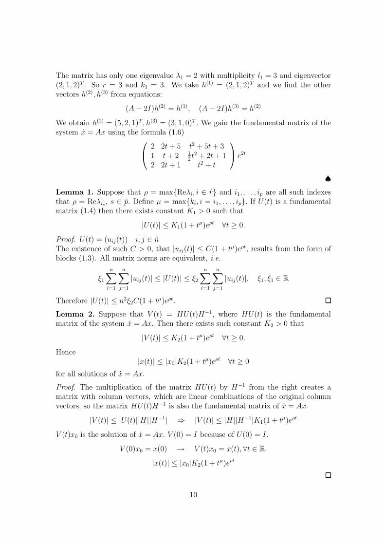
The matrix has only one eigenvalue λ1 = 2 with multiplicity l1 = 3 and eigenvector(2, 1, 2)T . So r = 3 and k1 = 3. We take h(1) = (2, 1, 2)T and we find the othervectors h(2), h(3) from equations:

(A− 2I)h(2) = h(1), (A− 2I)h(3) = h(2)

We obtain h(2) = (5, 2, 1)T , h(3) = (3, 1, 0)T . We gain the fundamental matrix of thesystem x = Ax using the formula (1.6)

2 2t+ 5 t2 + 5t+ 31 t+ 2 1

2t2 + 2t+ 1

2 2t+ 1 t2 + t

e2t

♠Lemma 1. Suppose that ρ = maxReλi, i ∈ r and i1, . . . , ip are all such indexesthat ρ = Reλis, s ∈ p. Define µ = maxki, i = i1, . . . , ip. If U(t) is a fundamentalmatrix (1.4) then there exists constant K1 > 0 such that

|U(t)| ≤ K1(1 + tµ)eρt ∀t ≥ 0.

Proof. U(t) = (uij(t)) i, j ∈ n

The existence of such C > 0, that |uij(t)| ≤ C(1 + tµ)eρt, results from the form ofblocks (1.3). All matrix norms are equivalent, i.e.

ξ1

n∑

i=1

n∑

j=1

|uij(t)| ≤ |U(t)| ≤ ξ2

n∑

i=1

n∑

j=1

|uij(t)|, ξ1, ξ1 ∈ R

Therefore |U(t)| ≤ n2ξ2C(1 + tµ)eρt.

Lemma 2. Suppose that V (t) = HU(t)H−1, where HU(t) is the fundamentalmatrix of the system x = Ax. Then there exists such constant K2 > 0 that

|V (t)| ≤ K2(1 + tµ)eρt ∀t ≥ 0.

Hence|x(t)| ≤ |x0|K2(1 + tµ)eρt ∀t ≥ 0

for all solutions of x = Ax.

Proof. The multiplication of the matrix HU(t) by H−1 from the right creates amatrix with column vectors, which are linear combinations of the original columnvectors, so the matrix HU(t)H−1 is also the fundamental matrix of x = Ax.

|V (t)| ≤ |U(t)||H||H−1| ⇒ |V (t)| ≤ |H||H−1|K1(1 + tµ)eρt

V (t)x0 is the solution of x = Ax. V (0) = I because of U(0) = I.

V (0)x0 = x(0) → V (t)x0 = x(t), ∀t ∈ R.

|x(t)| ≤ |x0|K2(1 + tµ)eρt

10

Theorem 2. 1.The stationary point x = 0 of the system x = Ax is Liapounovstable iff all eigenvalues of the matrix A have non-positive real parts, and moreoverthe lengths of chains respective to eigenvalues with zero real part are always one.2.The stationary point x = 0 of x = Ax is asymptotically stable iff all eigenvaluesof the matrix A have negative real parts.

Proof. 1. First we prove that the stationary point x = 0 of the system x = Ax isLiapounov stable iff the solution x(x0, t) is bounded for all initial values x0 ∈ R

n

and for all t ≥ 0.Suppose that all solutions x(x0, t) are bounded for all t ≥ 0. Therefore the fun-

damental matrix V (t) must be also bounded, i.e. ∃K > 0 |V (t)| ≤ K.

Choose ǫ > 0 and such initial condition x0 that |x0| < δ.

|x(x0, t)| = |V (t)x0| ≤ |V (t)||x0| < Kδ.

For a special choice of δ = ǫK

, the condition for Liapounov stability of the stationarypoint x = 0 is fulfilled.

Assume that the stationary point x = 0 is Liapounov stable, i.e.

∀ǫ > 0 ∃δ > 0 |x0| < δ ⇒ |x(x0, t)| < ǫ ∀t ≥ 0.

Suppose that there exists such x0 ∈ Rn that the solution x(x0, t) is not bounded for

t ≥ 0.Let us take y0 = δ

2|x0|x0. (It is correct because x0 cannot be 0.)

x(y0, t) = V (t)y0 =δ

2|x0|V (t)x0 =

δ

2|x0|x(x0, t) ∀t ≥ 0

Therefore the solution x(y0, t) is also unbounded although |y0| < δ and its normmust be less than ǫ from presumptions.

For this reason, it is enough to show that all solutions of x = Ax are boundedinstead of they are Liapounov stable.

Suppose that Reλi ≤ 0 ∀i ∈ r and if Reλj = 0 then kj = 1 for all such j. Wehave verified that |x(t)| ≤ |x0|K(1 + t) (lemma 2). So the solution could becomeunbounded as t→ ∞. However, all column vectors v(i)(t) of the fundamental matrixHU(t) satisfy that limt→∞|v(i)(t)| < ∞. Hence all solutions (which are some linearcombination of the column vectors v(i)(t)) must be bounded.

Assume that the previous condition for the eigenvalues is not true. So there existssuch s ∈ r that Reλs > 0 or Reλs = 0 but ks > 1. It is evident that if Reλs > 0then some solutions of x = Ax are unbounded. If Reλs = 0 and ks > 1 then thenorm of the respective column vector v(k1+kj−1+2) tends to infinity as t→ ∞. Hencethe statement 1 is proved.

2. Suppose that Reλi < 0 ∀i ∈ r. Using the previous lemma, we get

|x(t)| ≤ |x0|K2(1 + tµ)eρt.

11

So |x(t)| → 0 as t → ∞ and the condition for asymptotic stability of x = 0 isfulfilled.

Suppose that |x(t)| → 0 as t → ∞. This condition is satisfied when x(t) → 0.All eigenvalues must have negative real parts to fulfill x(t) → 0 as can be seen fromthe form of fundamental matrix (1.4).

Previous theorem is very useful but calculating the roots of characteristic polyno-mial analytically is very tedious and often impossible. Furthermore, the analyticalform of roots of a polynomial with parameters is often so complicated that we areunable to gain any information from it. Fortunately for purposes of determinationthe stability, this problem can be obviated as the following two theorems show.

Theorem 3. Consider the polynomial

Pn(x) = a0 +a1x+ . . .+anxn, n ≥ 1, a0 > 0, an 6= 0, ai ∈ R ∀i ∈ n. (1.7)

If all roots of this polynomial have negative real parts (such a polynomial is oftencalled Hurwitz’s polynomial), then all coefficients ai, i ∈ 0, . . . , n are positive.

Proof. Assume that xj = −αj ± iβj (j ∈ p) are complex roots of polynomial (1.7)and xk = −γk (k ∈ q) are the real ones. The polynomial is Hurwitz’s, so αj > 0∀j ∈ p, γk > 0 ∀k ∈ q. Denote the multiplicity of a root xk = −γk as mk andmultiplicity of xj = −αj + iβj as nj . The polynomial (1.7) have real coefficients soxj = −αj − iβj has the same multiplicity. It is obvious that

p∑

j=1

2nj +

q∑

k=1

mk = n.

All polynomials can be written in the form:

Pn(x) = an

p∏

j=1

(x+ αj − iβj)nj(x+ αj + iβj)

nj

q∏

k=1

(x+ γk)mk

Pn(x) = an

p∏

j=1

(x2 + 2αjx+ βj2 + αj

2)nj

q∏

k=1

(x+ γk)mk

If we compare the coefficients of terms with the same order of x we see that all coef-ficients ai have the same sign. So all coefficients must be positive as a consequenceof positivity of a0.

The roots of polynomial P2(x) = a2x2 +a1x+a0 are either real or it is a complex

conjugated pair. If a0, a1, a2 > 0 then the complex conjugated pair has a negativereal part. For the same reason both the real roots are negative as results fromViete´s formulas for roots of a quadratic equation. The roots of polynomial P3(x) =x3 +x2 +4x+30 are −3, 1+3i, 1−3i. So, the previous condition is necessary but notsufficient for polynomials of the order grater than two. For this reason, we wouldlike to know another criterion that will be both necessary and sufficient. Beforewriting this criterion,we introduce some important properties of polynomials.

12

Definition 8. Polynomial

F (x) = (1 + αx)f(x) + f(−x), α > 0 (1.8)

is called a conjugated polynomial to the polynomial f(x).

Lemma 3. The polynomial (1.8) conjugated to the Hurwitz’s polynomial f(x) isalso the Hurwitz’s polynomial.

Proof. Consider the polynomials Φm(x) = (1+αx)f(x)+mf(−x), where 0 ≤ m ≤ 1.The polynomial f(x) = a0 + a1x+ . . .+ anx

n is Hurwitz’s from the assumptions soa0, a1, . . . , an > 0. Then

Φm(x) = (1 + αx)(a0 + a1x+ . . .+ anxn) +m(a0 − a1x+ . . .+ an(−1)n

xn) (1.9)

Therefore, the coefficients ami are linear functions of the parameter m and moreover

the roots of this polynomial are closed in a sufficiently large circle (αan > 0 ⇒|Φm(x)| > 0 |x| ≥ R), where R does not depend on m.

The polynomial Φ0(x) = (1 + αx)f(x) is the Hurwitz’s polynomial because ofpositivity of α. We use the absurdum proof to show that Φm are Hurwitz’s poly-nomials for all m ∈ 〈0, 1〉. Assume that m ∈ 〈0, 1〉 is such a parameter that thepolynomial Φm is not the Hurwitz’s polynomial. The roots of (1.9) are continuousbounded functions of the parameter m so there exists such m ∈ 〈0, 1〉 that at leastone root of the polynomial Φm leaves the left half-plane of the complex plane torealize that Φm is not the Hurwitz’s polynomial. Therefore Φm has an imaginaryroot iβ.

Φm(iβ) = (1 + iαβ)f(iβ) + mf(−iβ) = 0

|1 + iαβ||f(iβ)| = m|f(−iβ)| (1.10)

f(x) = f(x) for all polynomials with real coefficients.

|f(−iβ)| = |f(iβ)| = |f(iβ)| = |f(iβ)|

|f(iβ)| 6= 0 because f is Hurwitz’s polynomial so we can cancel it out from (1.10).

|1 + iαβ| = m ⇒ 1 + α2β2 = m2

Hence m > 1 (α > 0, β 6= 0) and it is against the condition m ∈ 〈0, 1〉. Soall polynomials Φm(x) are the Hurwitz’s polynomials for all m ∈ 〈0, 1〉 and thestatement is proved (for special choice m = 1).

Lemma 4. For all Hurwitz’s polynomials F (x) of the order n+1 there exists α > 0and Hurwitz’s polynomial f(x) of the order n such that

F (x) = (1 + αx)f(x) + f(−x). (1.11)

13

Proof.

F (−x) = (1 − αx)f(−x) + f(x) (1.12)

We compare the terms f(−x) from equations (1.11) and (1.12) and we gain thepolynomial f(x) as a function of F (x) this way.

α2x2f(x) = (αx− 1)F (x) + F (−x) (1.13)

Suppose that F (x) = A0 + A1x+ . . .+ An+1xn+1, A0, . . . , An+1 > 0. Therefore

α2x2f(x) = A0αx− 2A1x+ A1αx2 + . . .

Thus f(x) is the polynomial of the order n and the condition (1.11) is fulfilled forspecial choice α = 2A1

A0

. We prove that f(x) is also the Hurwitz’s polynomial usinga similar trick as in the previous lemma.

Consider polynomials

Φm(x) = (αx− 1)F (x) +mF (−x), m ∈ 〈0, 1〉. (1.14)

The roots of the polynomial (1.14) are continuous bounded functions of the param-eter m. The polynomial Φ0(x) = (αx− 1)F (x) has n+ 1 roots in the left half of thecomplex plane and xn+2 = 1

αis in the right one.

The roots of (1.14) are placed this way for all values of the parameter m ∈ 〈0, 1).The curve xi = xi(m) must intersect the imaginary axis to cross to the other half-plane. However, it is impossible for m ∈ 〈0, 1). The prove is identical as in theprevious lemma so we would not give it here again.

We know that the polynomials Φm(x) have n+1 roots with negative real part andone with positive real part for m ∈ 〈0.1). However, the polynomial Φ1(x) (m = 1)has two null roots. Suppose that xl(m) → 0 and xk(m) → 0 as m → 1 − . We usethe relation between the polynomial a0 + . . .+ anx

n and its roots:∑n

j=11xj

= −a1

a0

.

n+2∑

j=1

1

xj(m)=A1

A0

(1.15)

as results from the form of Φm(x). Therefore one of the roots xk(m), xl(m) musthave positive real part. If not, the left part of the equation (1.15) would tend to−∞ and the right part would remain positive and it is impossible.

Hence Φ1(x) = (αx− 1)F (x) + F (−x) has two null roots (the coefficient, whichstands before the term x2, is positive) and n roots with negative real part. α2x2f(x) =(αx− 1)F (x) + F (−x) and therefore f(x) is really the Hurwitz’s polynomial.

Definition 9. Consider the polynomial

Pn(x) = a0 + a1x+ . . .+ anxn, n ≥ 1, ai > 0 ∀i ∈ 0, . . . , n. (1.16)

14

The matrix

a1 a0 0 0 . . . 0a3 a2 a1 a0 . . . 0...

......

.... . .

a2n−1 a2n−2 a2n−3 a2n−4 . . . an

,

where aj = 0 for j < 0 and j > n, is called the Hurwitz’s matrix of the polynomialPn(x) = a0 + a1x+ . . .+ anx

n.

Theorem 4 (Hurwitz’s criterion). All roots of polynomial (1.16) have negativereal parts iff all main minors of the Hurwitz’s matrix are positive, i.e.

D1 = a1 > 0

D2 = det

(

a1 a0

a3 a2

)

> 0

...

Dn = anDn−1 > 0.

Proof. 1. ⇒ We prove it using the mathematical induction.

n = 1 f(x) = a0 + a1x⇒ x = −a0

a1< 0 ⇒ ∆1 = a1 > 0

Suppose that the theorem is true for all Hurwitz’s polynomials of the order n andF (x) is the Hurwitz’s polynomial of the order n + 1. F (x) can be written as aconjugated polynomial to the Hurwitz’s polynomial of the order n. F (x) = (1 +2cx)f(x) + f(−x), where c > 0 and f(x) = a0 + . . .+ anx

n.

F (x) = (1 + 2cx)(a0 + a1 + . . .+ anxn) + (a0 − a1x+ . . .+ (−1)n

anxn)

F (x) = 2a0 + 2n∑

k=1

(cak−1 +1 + (−1)k

2ak)x

k + 2ancxn+1

So the main minors of the Hurwitz’s matrix look like

Dk+1 = 2k+1

∣

∣

∣

∣

∣

∣

∣

∣

∣

ca0 a0 0 0 . . . 0ca2 ca1 + a2 ca0 0 . . . 0...c2k ca2k−1 + a2k ca2k−2 . . .

∣

∣

∣

∣

∣

∣

∣

∣

∣

Dk+1 = 2k+1ck+1

∣

∣

∣

∣

∣

∣

∣

∣

∣

a1 a0 0 0 . . . 0a3 a2 a1 a0 . . . 0...

......

.... . .

a2n−1 a2n−2 a2n−3 a2n−4 . . . an

∣

∣

∣

∣

∣

∣

∣

∣

∣

= αk+1a0∆k

15

∆k is the main minor of the Hurwitz’s matrix of the polynomial f(x). We knowthat a0, α and ∆k are positive from premises so Dk+1 is also positive.

2.⇐

n = 1 f(x) = a0 + a1x a0 > 0 ∆1 = a1 > 0 ⇒ x = −a0

a1< 0

Suppose that the statement is true for all Hurwitz’s polynomials of the order n,F (x) = A0 +A1x+ . . .+An+1x

n+1 and A0 > 0, D1 = A1 > 0, . . . , Dn+1 > 0. We canimagine polynomial F (x) as the conjugated one to f(x) = a0 + . . . + anx

n (a0 >

0, an 6= 0). Dk+1 = αk+1a0∆k > 0 from the premises and proved part of the theorem.

α > 0 ⇒ ∆k > 0 k ∈ n

Thus f(x) is Hurwitz’s polynomial and therefore F (x) is also Hurwitz’s one as aresult of lemma 3.

Example 6. Consider a linear system of differential equations with real parametersp, q.

x1 = −x1 + px2

x2 = qx1 − x2 + px3 (1.17)

x3 = qx2 − x3.

We determine the values of p, q, for which the null solution of (1.17) is asymptoticallystable.

First we find the eigenvalues of the respective matrix A, the characteristic poly-nomial of the matrix A is

det(A− λI) = −(λ+ 1)(λ2 + 2λ+ 1 − 2pq) ⇒ λ1 = −1 λ2,3 = −1 ±√

2pq.

Therefore the null solution of the system (1.17) is asymptotically stable iff pq < 12.

The theorem 3 is necessary and sufficient when looking for the roots with negativereal parts of the equation λ2 + 2λ+ 1 − 2pq. So 1 − 2pq > 0 ⇒ pq < 1

2.

Finally, we use the Hurwitz’s criterion to examine the asymptotic stability of thenull solution of (1.17). det(A− λI) = λ3 + 3λ2 + (3− 2pq)λ+ 1− 2pq. We do knowthat λ1 = −1, but the application of the Hurwitz’s criterion for polynomials of theorder less than three loses the sense.

First we must satisfy the necessary condition to create the Hurwitz’s matrix(ai > 0 i ∈ 0, 1, 2, 3). Hence pq < 1

2. So the Hurwitz’s matrix has the following

form for such parameters p, q that pq < 12

:

3 − 2pq 1 − 2pq 01 3 3 − 2pq0 0 1

16

D1 = 3 − 2pq > 0 ⇒ pq <3

2D2 = 8 − 4pq > 0 ⇒ pq < 2

D3 = 1D2 > 0 ⇒ D2 > 0

Therefore pq < 12. This example illustrates the fact that we must not forget the

condition for positivity of the respective polynomial coefficients. Without this con-dition, the Hurwitz’s criterion need not to give us the right results. ♠

1.4 Linearization of nonlinear systems

We have spent plenty of time investigating the stability of solutions of the systems oflinear differential equations, although the most of dynamical systems are describedby the nonlinear ones. The question arises whether it was a waste of time and energyor not.

Theorem 5. Suppose that

x = Ax+ g(x), g(0) = 0, (1.18)

where A ∈ Rn,n and g is a vector function, which is continuous in some domain

H ∈ Rn (0 ∈ H) and moreover g satisfies the condition

lim|x|→0|g(x)||x| = 0. (1.19)

Then:1. If all eigenvalues of A have negative real parts the stationary point x = 0 of

the system (1.18) is asymptotically Liapounov stable.2. If there exists at least one eigenvalue of the matrix A with positive real part

then the stationary point x = 0 is Liapounov unstable.

We need three simple but useful lemmas to prove this theorem.

Lemma 5. Suppose that functions φ(t) and ψ(t) have derivatives in an intervalI = (a, a + b) (b > 0) and φ(t) < ψ(t) for all t ∈ (a, a + ǫ), where b > ǫ > 0. Thenthere occurs one of the following cases:

1.φ(t) < ψ(t) ∀t ∈ I

2.There exists t0 ∈ I such that φ(t) < ψ(t) ∀t ∈ (a, t0), φ(t0) = ψ(t0) andφ(t0) ≥ ψ(t0).

Proof. The possibility, that case 1 occurs, is obvious. Suppose that 1 is not true.Then there exists minimal t0 > a such that φ(t0) = ψ(t0). Moreover for all h > 0,φ(t0 − h) < ψ(t0 − h). Hence

φ(t0) − φ(t0 − h)

h>ψ(t0) − ψ(t0 − h)

h.

We get the case 2 for h→ 0.

17

Lemma 6. Suppose that all eigenvalues λi (i ∈ n) of the matrix A ∈ Rn,n satisfy

the condition Reλi < α. Then |eAt| ≤ ceαt for all t ≥ 0 and convenient constant c.

Proof. From the previous, we know that the differential equation x = Ax has nlinearly independent solutions in the form: x(t) = eλtp(t), where λ is the eigenvalueof the matrix A and p(t) = (p1(t), . . . , pn(t))

T is a vector, which components arepolynomials of the order ≤ n. Denote α − Reλ as β. |pi(t)| ≤ cie

βt because ofpositivity of β. Hence

|eλtpi(t)| ≤ eβ+Reλtci = cieαt

Lemma 7. Suppose that I is such an interval that t0 ∈ I and γ is a positiveconstant. Suppose that functions ξ, φ : I → R are continuous and nonnegative in I

and moreover:

ξ(t) ≤ γ +∣

∣

∣

∫ t

t0

ρ(τ)ξ(τ)dτ∣

∣

∣t ∈ I (1.20)

Thenξ(t) ≤ γe

|∫ t

t0ρ(τ)dτ |

t ∈ I.

Proof. We prove it for t ≥ t0, for t < t0, the proof is analogous.

ρ(t)ξ(t)

γ +∫ t

t0ρ(τ)ξ(τ)dτ

≤ ρ(t) t ≥ t0

as results from (1.20). We integrate both sides of the previous equation:

ln(γ +

∫ t

t0

ρ(τ)ξ(τ)dτ) − lnγ ≤∫ t

t0

ρ(τ)dτ

ξ(t) ≤ γ +

∫ t

t0

ρ(τ)ξ(τ)dτ ≤ γe∫ t

t0ρ(τ)dτ

Proof of the theorem 5. 1. From the lemma 6, we know that there exist c > 1, β > 0such that Reλi < −β and |eAt| ≤ ce−βt for t ≥ 0. The condition (1.19) implies:

∃δ > 0 |x| < δ ⇒ |g(x)| < β

2c|x|.

We want to show that if the norm x0 is sufficiently small, then the norm of thesolution of (1.18) with initial condition x0 tends to zero.

All solutions of the equation (1.18) with initial condition x(0) = x0 can be writtenin the form:

x(t) = eAtx0 +

∫ t

0

eA(t−τ)g(x(τ))dτ.

18

Hence if |x(t)| ≤ δ

|x(t)| ≤ |x0|ce−βt +

∫ t

0

β

2e−β(t−τ)|x(τ)|dτ.

Suppose that |x0| < ǫ and φ(t) = |x(t)|eβt.

φ(t) ≤ cǫ+β

2

∫ t

0

φ(τ)dτ

Using the previous lemma, we get φ(t) ≤ cǫeβt/2 ⇔ |x(t)| ≤ cǫe−βt

2 .2. We transfer the equation (1.18) in a more convenient form. Suppose that

the matrix H transfers the matrix A to its Jordan normal form Q (Q = H−1AH).Assume that α > 0 and the matrix B is a diagonal matrix B = diag(α, α2, . . . , αn).It is easy to see that B−1 = diag(α−1, . . . , α−n).

By using the substitution x(t) = HBy(t), we get the equation (1.18) in the form:

y = B−1H−1(AHBy + g(HBy)), whereB−1H−1AHB = B−1QB := C

y = Cy + f(y) wheref(y) = B−1H−1g(HBy). (1.21)

The matrix C = B−1QB ⇔ dii = λi di,i+1 = 0 or α as results from the form ofnormal Jordan matrix Q.

We would like to know if the function f(y) also satisfies the condition (1.19).

lim|x|→0|g(x)||x| = 0 ⇔ (∀ǫ > 0)(∃δ > 0)(|x| < δ ⇒ |g(x)| < ǫ|x|).

|f(x)| = |B−1H−1g(HBx)| ≤ |B−1H−1|ǫ|HB||x| for|x| < |HB|δHence f(x) has similar properties as g(x) for sufficiently small x.

Let us write the equation (1.21) in the components:

yi = λiyi + [αyi+1] + fi(y) i ∈ n. (1.22)

From the form of the matrix C, or if you like Q, we know that the term in squarebrackets is nonzero iff i denotes a Q matrix row in the matrix cell of the order graterthan 1 and moreover it is not the last such row.

Denote as j(k) all such indexes, for which Reλj > 0 (λk ≤ 0) and define thefunctions φ(t) =

∑nj=1 |yj(t)|2 and ψ(t) =

∑nk=1 |yk(t)|2, where y(t) is the solution

of (1.21). We choose such α > 0 that 0 < 6α < Reλj ∀j and δ > 0 so small that itsatisfies: |f(y)| < α|y| for |y| < δ.

Suppose that y(t) is a solution with initial conditions:

|y(t0)| < δ ψ(t0) < φ(t0). (1.23)

If |y(t)| ≤ δ and ψ(t) ≤ φ(t) we can write:

19

φ(t) =n∑

j=1

(yj(t)yj(t) + yj(t)yj(t)) = 2n∑

j=1

Re(yj(t)yj(t))

Using the relation (1.22), we get:

φ(t) = 2n∑

j=1

Re(λjyj(t)yj(t) + [αyj+1(t)yj(t)] + yj(t)fj(y(t))) (1.24)

Let us look at the particular components in a more detail.

n∑

j=1

Re(λjyj(t)yj(t)) =

n∑

j=1

Reλj |yj(t)|2 > 6αφ(t) (1.25)

n∑

j=1

Re(yj+1(t)yj(t)) ≤n∑

j=1

|yj(t)yj+1(t)| ≤

√

√

√

√

n∑

j=1

|yj(t)|2.n∑

j=1

|yj(t)|2 = φ(t) (1.26)

The last but one step results from the Schwartz inequality.

n∑

j=1

Re(yj(t)fj(y(t))) ≤

√

√

√

√

n∑

j=1

|yj(t)|2.n∑

j=1

|fj(y(t))|2 ≤√

φ(t)|fj(y(t))| ≤ 2αφ(t)

(1.27)The last inequality is a consequence of the following:

|f(y(t))| ≤ α|y(t)| ≤ α√

φ(t) + ψ(t) ≤ 2α√

φ(t)

Hence1

2φ(t) > 6αφ(t) − αφ(t) − 2αφ(t) = 3αφ(t). (1.28)

The relation (1.24) is also true for ψ(t) but we must not forget that Reλk ≤ 0.

n∑

j=1

Re(λjyj(t)yj(t)) ≤ 0

n∑

j=1

Re(yj+1(t)yj(t)) ≤ αψ(t)

n∑

j=1

Re(yj(t)fj((y(t)))) ≤ 2αφ(t)

20

Hence 12ψ(t) ≤ αψ(t) + 2αφ(t). We have assumed that ψ(t) ≤ φ(t). We summarize

the previous :

φ(t) > 6αφ(t)

ψ(t) ≤ 2αψ(t) + 4αφ(t) ≤ 6αφ(t) < φ(t).

Moreover, ψ(t0) < φ(t0). As a consequence of lemma 5, we see that ψ(t) < φ(t).All solutions y(t), which satisfy the initial condition (1.23) and moreover |y(t)| ≤ δ,fulfill also ψ(t) < φ(t) and φ(t) > 6αφ(t). Hence φ(t) ≥ φ(t0)e

6αt and thereforefor all such solutions, there exists such t1 that |y(t1)| = δ. The stationary solutiony(t) = 0 cannot be Liapounov stable.

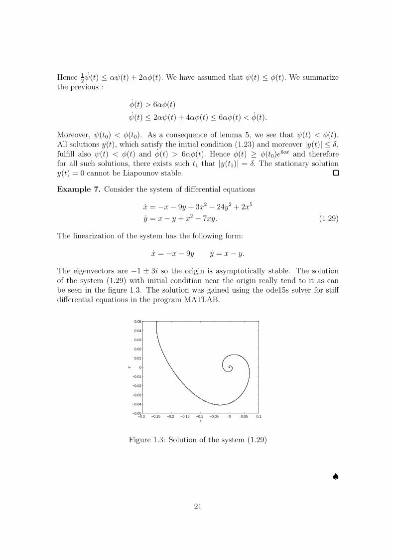
Example 7. Consider the system of differential equations

x = −x− 9y + 3x2 − 24y2 + 2x5

y = x− y + x2 − 7xy. (1.29)

The linearization of the system has the following form:

x = −x− 9y y = x− y.

The eigenvectors are −1 ± 3i so the origin is asymptotically stable. The solutionof the system (1.29) with initial condition near the origin really tend to it as canbe seen in the figure 1.3. The solution was gained using the ode15s solver for stiffdifferential equations in the program MATLAB.

−0.3 −0.25 −0.2 −0.15 −0.1 −0.05 0 0.05 0.1−0.05

−0.04

−0.03

−0.02

−0.01

0

0.01

0.02

0.03

0.04

0.05

x

y

Figure 1.3: Solution of the system (1.29)

♠

21

Chapter 2

Bifurcations

The word bifurcation denotes a situation in which the solutions of a nonlinear systemof differential equations alter their character with a change of a parameter on whichthe solutions depend. Bifurcation theory studies these changes (e.g. appearanceand disappearance of the stationary points, dependence of their stability on theparameter etc.)

In this chapter, we use the stationary solutions of some simple differential equa-tions to describe the most important types of bifurcations. We prefer the heuristicapproach to the rigorous mathematical description, that can be found in e.g. [4] or[1].

2.1 Transcritical bifurcation

Let us take the first-order differential equation:

dx

dt= x(a− c− abx) (2.1)

with positive constants b, c. We try to show how the stability of stationary pointsdepends on the parameter a.

This equation has two stationary points:

x = 0 ∀a ∈ R x =a− c

ab∀a ∈ R \ 0

In order to investigate the stability of the null solution, we linearize the equation(2.1):

dx

dt= (a− c)x.

It is not too difficult to see that its solution is:

x(t) = x0e(a−c)t, where x0 = x(0).

22

Thus the null solution is stable for a < c and unstable for a > c. The linearizedsystem is not able to determine the stability of the null solution in case a = c.

Fortunately, this equation is simply soluble.

dx

dt= −abx2 − 1

x2

dx

dt= ab

dx−1

dt= ab

x−1(t) = abt+ x0−1 x(t) =

x0

x0abt+ 1

We see that x(t) → ∞ as t→ − 1abx0

, so the null solution is unstable for a = c.

To examine the stability of the stationary solution x = a−cab

, we change the co-ordinates in order to arrange x = a−c

abto the origin. We may similarly as in the

previous case show that the solution x = a−cab

is stable for c < a and unstable forc ≥ a.

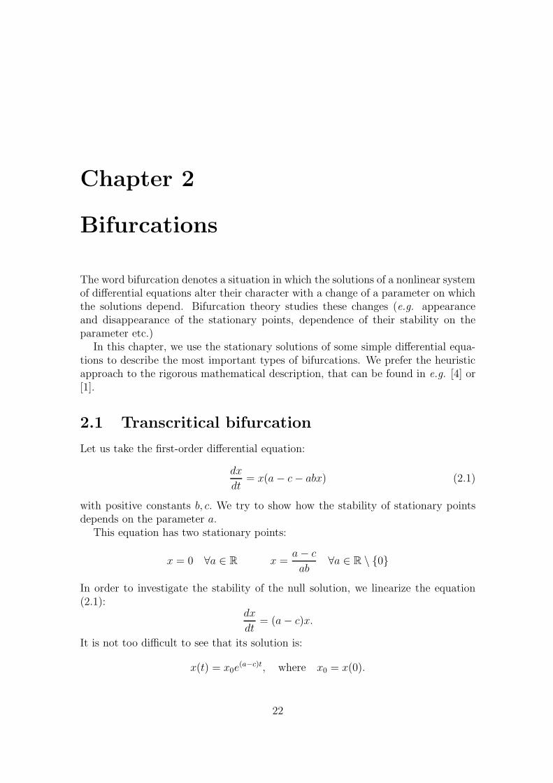
We plot the stationary points versus the value of a parameter a in so called bifur-cation diagram - figure 2.1 (the diagram is drawn for c = b = 1). It is conventionalto draw the stable solutions as continuous curves and the unstable ones as dashedcurves.

−3 −2 −1 0 1 2 3 4 5 6 7 8

−8

−6

−4

−2

0

2

4

6

8

10

a

x

Transcritical bifurcation

Figure 2.1: Transcritical bifurcation

The situation for a = c is called a transcritical bifurcation. It occurs when onestable and one unstable fixed points cross each other. At the crossing point theyexchange their stability property. So the stable stationary point becomes unstableand vice versa.

23

2.2 Saddle-node bifurcation

The number of stationary points of the differential equation

dx

dt= a− x2 (2.2)

depends on the value of the parameter a. There are two fixed points for a > 0, onefixed point for a = 0 and none for a < 0.

Take the stationary solution x = A, A := ±√a for a > 0. By changing the

coordinates (y = x− A) we obtained the differential equation

dy

dt= −y2 − 2Ay.

We can linearize it for the null solution:

dy

dt= −2Ay y = y0e

−2At

So the solution x = A is stable for A > 0 and ustable for A < 0.To determine the stability of the solution x = 0, we must solve the equation (2.2)

explicitly. Similar equation was solved in previous section. So its solution is:

x =x0

1 + x0t

and it is unstable.Now we do know that the stationary points x =

√a are stable for ∀a > 0 and

the stationary points x = −√a are unstable for ∀a ≥ 0. That is all that we need for

plotting the bifurcation diagram - figure 2.2.The situation at the origin is called a saddle-node bifurcation and occurs when a

stable fixed point (a node) collides and annihilates with an unstable one (a saddle).

2.3 Pitchfork bifurcation

Consider the differential equation

dx

dt= ax− bx3, a, b ∈ R. (2.3)

The equilibrium points are x = 0 ∀a and x = ±√

ab∀a, b such that a

b> 0. To

determine the stability of the null solution, we take the linearized system: dxdt

= ax

with solution x(t) = x0eat. It is obvious that the null solution is stable for a < 0 and

unstable for a > 0. The linear criterion is not sufficient in case a = 0 and we haveto solve the equation (2.3) explicitly.

dx

dt= −bx3 − 1

x3

dx

dt= b

dx−2

dt= 2b

24

−1 0 1 2 3 4 5 6 7−3

−2

−1

0

1

2

3Saddle−node bifurcation

a

x

Figure 2.2: Saddle-node bifurcation

x−2(t) = 2bt+ x0−2 x2(t) =

x02

1 + 2btx02

x(t) =√

x2(t)sgnx0

So the solution x = 0 is stable for b > 0 and unstable for b < 0.To investigate the stability of the solution x = ±

√

ab, we change the coordinates

again and we obtain this linearized system for the null solution dydt

= −2ay with solu-tion y(t) = e−2at. We say that the stationary points x = ±

√

ab

are stable (unstable)for a > 0 (a < 0) on account of this solution.

We obtain two different bifurcation diagrams for b > 0 (figure 2.3) and b < 0(figure 2.4).

−2 −1 0 1 2 3 4 5 6 7−3

−2

−1

0

1

2

3Supercritical pitchfork bifurcation

a

x

Figure 2.3: Supercritical pitchfork bifurcation

25

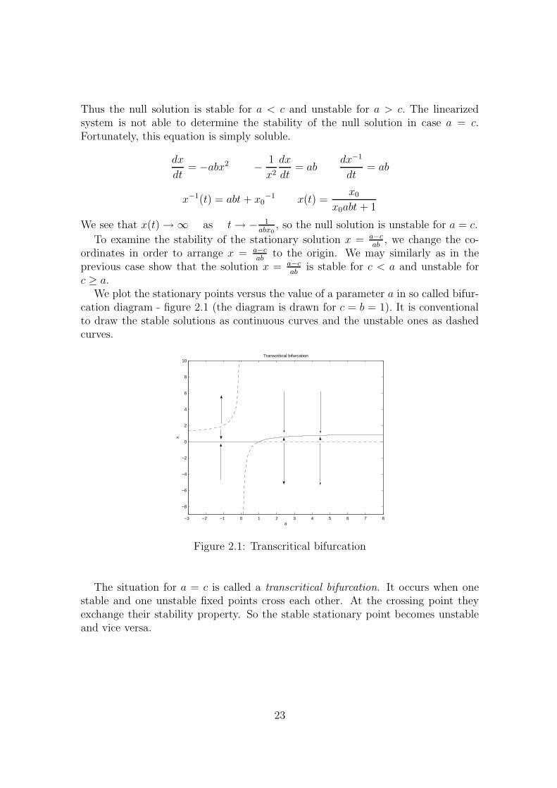
There is a unique stationary point x = 0 for a ≤ 0 but three fixed points fora > 0. The bifurcated solutions x = ±

√

ab

are stable whenever they exist and theyappear as the parameter a increases above its critical value. It is called supercritical

pitchfork bifurcation. The name pitchfork is not much surprising considering theappearance of the bifurcation.

−7 −6 −5 −4 −3 −2 −1 0 1 2−3

−2

−1

0

1

2

3

a

x

Subcritical pitchfork bifurcation

Figure 2.4: Subcritical pitchfork bifurcation

The situation for b < 0 is similar to the previous case, but the bifurcated solutionsx = ±

√

ab

arise as a decreases underneath its critical value and they are unstablewhenever they exist. This bifurcation is called a subcritical pitchfork bifurcation.

2.4 Hopf bifurcation

We have seen that the stationary point loses its stability when the eigenvalue crossesthe imaginary axis (the control parameter must increase or decrease its criticalvalue). We know that the eigenvalue can be a complex number. In this case, theconjugated pair of eigenvalues crosses the imaginary axis together. This phenomenonis called a Hopf bifurcation.

It is obvious that the phase space must be at least two-dimensional in order forHopf bifurcation to occur.

Consider the system of differential equations

x = ax− by − (x2 + y2)x

y = bx+ ay − (x2 + y2)y, (2.4)

where a, b are real parameters. The origin is a stationary point and we try toinvestigate its stability. The linearization of the system (2.4) has the following form:

x = ax− by y = bx+ ay.

26

The eigenvalues are a ± ib. Therefore the origin is stable for a < 0 and unstablefor a > 0. We expect that some bifurcation occurs when a = 0 (similarly as in theprevious examples). We use polar coordinates (x = rcosϕ, y = rsinϕ) to solve thesystem (2.4) explicitly. We see that x+ iy = reiϕ. Hence

d(reiϕ)

dt=dx

dt+ i

dy

dtd(reiϕ)

dt=(dr

dt+ ir

dϕ

dt

)

eiϕ

dx

dt+ i

dy

dt=ax− by − (x2 + y2)x+ ibx+ iay − i(x2 + y2)y = (ar − r3 + ibr)eiϕ.

We compare the real and imaginary parts

r = ar − r3 ϕ = b. (2.5)

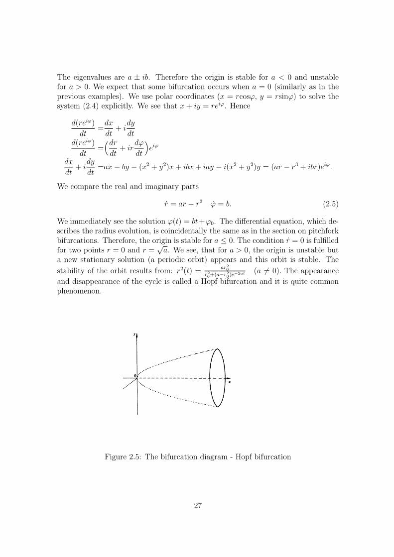
We immediately see the solution ϕ(t) = bt+ϕ0. The differential equation, which de-scribes the radius evolution, is coincidentally the same as in the section on pitchforkbifurcations. Therefore, the origin is stable for a ≤ 0. The condition r = 0 is fulfilledfor two points r = 0 and r =

√a. We see, that for a > 0, the origin is unstable but

a new stationary solution (a periodic orbit) appears and this orbit is stable. The

stability of the orbit results from: r2(t) =ar2

0

r2

0+(a−r2

0)e−2at (a 6= 0). The appearance

and disappearance of the cycle is called a Hopf bifurcation and it is quite commonphenomenon.

Figure 2.5: The bifurcation diagram - Hopf bifurcation

27

2.5 Classification of the stationary points

2.5.1 One-dimensional case

The phase space is just the x-axis in one-dimensional case and the time evolution ofthe point x0 is determined by the equation x = f(x). Until now, we have met stableand unstable stationary points. We will extend our knowledge about the stationarypoints in this section.

Suppose that x = a0 is a stationary point of the equation x = f(x). Take thepoint x = a0 + a, where a is sufficiently small, and look at the possible behaviour ofthis point.

We know the Taylor expansion of the function f(x) for x = a0 + a.

f(x) = f(a0) + af ′(a0) +a2

2f ′′(a0) + . . .

The first term on the right side is equal to zero by the definition of stationary point.The value of f ′ at a0 is called the eigenvalue of stationary point a0 (or often aLiapounov exponent) and it is denoted as λ = df

dx(a0).

Suppose that λ < 0. Then the point x decreases toward a0 from the right andincreases to a0 from the left. Therefore a0 attracts nearby trajectories. This type ofstationary points is called a node.

Assume that λ > 0. Then conversely, the trajectories move away from a0 on bothsides. Such stationary point is called a repellor.

Finally, λ = 0. This case is more difficult than the previous ones because thestationary point a0 can be both a node and a repellor, or the third possibility canoccur when the stationary point will attract trajectories on one side and repel themon the other. Such stationary point is called a saddle point.

When λ = 0 the first nonzero term is f ′′. The change of the sign of the secondderivative of f as x passes through a0 is necessary in order to a0 could be a repelloror a node. It is easy to see that the second derivative must be positive from the leftand negative from the right for the node.

The last possibility, when the second derivative has the same sign on both sidesof a0, is a saddle point. There can occur two cases: the sign of the derivative ispositive, such saddle point is called type I saddle point, and the sign is negative -type II saddle point. So the type I saddle point attract trajectories from the leftand repel them from the right.

There can exist more than one stationary point for equation x = f(x). Thesmoothness of the function f sets bounds for the types of the stationary points thatcan be placed nearby themselves. Let us take two repellors. It is obvious that theycannot neighbour and moreover the stationary point between them must be a node.Conversely, two nodes need a repellor between them.

Type I saddle point cannot lie nearby the type II saddle. The stationary pointbetween them is a node. Similarly, the type II saddle point and type I saddle point

28

must have a repellor between them. On the other hand, the saddle points of thesame type can have themselves as a neighbour.

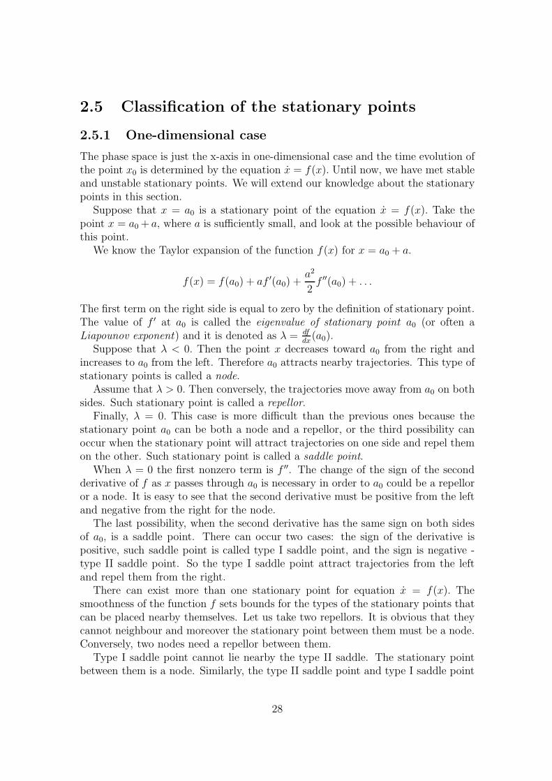
Example 8. Consider the equation x = cosx. We see that there exists infinitenumber of fixed points xk = (2k+ 1)π

2, where k ∈ Z. The same way as the values of

the Liapounov exponents -1 change for 1, the nodes change for the repellors. So wehave a never-ending chain of the repellors and nodes (figure 2.6).

−10 −8 −6 −4 −2 0 2 4 6 8 10

−0.8

−0.6

−0.4

−0.2

0

0.2

0.4

0.6

0.8

1

x

f(x)

N R N R N R

Figure 2.6: The stationary points of x = cos x

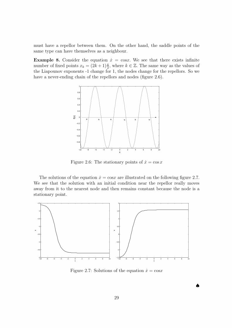
The solutions of the equation x = cosx are illustrated on the following figure 2.7.We see that the solution with an initial condition near the repellor really movesaway from it to the nearest node and then remains constant because the node is astationary point.

−10 −8 −6 −4 −2 0 2 4 6 8 10−5

−4.5

−4

−3.5

−3

−2.5

−2

−1.5

t

x

−10 −8 −6 −4 −2 0 2 4 6 8 10−1.5

−1

−0.5

0

0.5

1

1.5

2

t

x

Figure 2.7: Solutions of the equation x = cosx

♠

29

2.5.2 Two-dimensional case

We would like to extend previous considerations about stationary points to two-dimensional phase space. Suppose that

x1 = f1(x1, x2)

x2 = f2(x1, x2)

are the differential equations describing the dynamical system with a stationarypoint ~a0 = (a01, a02). Just as in one dimension, we expect that the type of stationarypoint ~a0 depends on the partial derivatives: ∂f1

∂x1

, ∂f1

∂x2

, ∂f2

∂x1

and ∂f2

∂x2

. The character ofthe dependence will be discussed in the following.

Let us again take the point ~x = (x1, x2), which is sufficiently close to the station-ary point ~a0, and write the Taylor expansion of the functions f1(x), f2(x).

f1(~x) = (x1 − a01)∂f1

∂x1(~a0) + (x2 − a02)

∂f1

∂x2(~a0) + . . . (2.6)

f2(~x) = (x1 − a01)∂f2

∂x1(~a0) + (x2 − a02)

∂f2

∂x2(~a0) + . . . (2.7)

We have omitted the terms f1(~a0), f2(~a0) because they are zero by the definition ofstationary point and ignored the derivatives of the order higher than the first. (Theanalysis, when ∂fi

∂xj= 0 i, j ∈ 2, is analogous as in the one-dimensional phase space

but we will be not do it here.)We introduce new variables y1 = x1 − a01, y2 = x2 − a02 that represent the

distance between the nearby point ~x and the stationary point ~a0. We have met anode, a repellor and a saddle point. We await that the distance tend to zero for anode and to infinity for a repellor. For a saddle point, we expect the different singsof the eigenvalues.

y1 =∂f1

∂x1(~a0)y1 +

∂f1

∂x2(~a0)y2

y2 =∂f2

∂x1(~a0)y1 +

∂f1

∂x1(~a0)y2. (2.8)

It is a system of differential equations with constant coefficients. We have familiar-ized ourselves with properties of its solutions in the first chapter. First, we mustcreate so-called Jacobian matrix J of the vector function f to find the eigenvaluesof system (2.8).

J =

(

∂f1

∂x1

∂f1

∂x2

∂f2

∂x1

∂f2

∂x2

)

, where the partial derivatives are evaluated at the stationary

point ~a0.

Using the terminology of the linear algebra, we obtain the eigenvalues in the form:

λ1,2 =TrJ ±

√

(TrJ)2 − 4detJ

2.

30

The solution of (2.8) is then:

y1(t) = c1h11e

λ1t + c2h21e

λ2t

y2(t) = c1h12e

λ1t + c2h22e

λ2t,

where ci ∈ R and h(i) is the eigenvector respective to eigenvalue λi, i ∈ 2.First, we assume that the eigenvalues are real, i.e.

(TrJ)2 − 4detJ ≥ 0 ⇔ detJ ≤ 1

4(TrJ)2

If detJ < 0 the eigenvalues have opposite signs and hence the stationary point is asaddle.

Both eigenvalues must be negative (positive) for ~a0 to be a node (a repellor).Therefore TrJ < 0 (TrJ > 0) and detJ > 0 in both cases.

Let us discuss the complex eigenvalues, i.e. detJ > 14(TrJ)2

. If we denote Tr2J as

a and

√(TrJ)2−4detJ

2as b, we can write the solution in the form:

yj(t) =eat

2(c1h

1je

ibt + c2h2je

−ibt), j ∈ 2.

We see that yj(t) oscillates with increasing (a > 0) or decreasing (a < 0) amplitude.Therefore if TrJ < 0 then the points in a neighbourhood of ~a0 tend to it on thespiral and ~a0 is called a spiral node. Analogously, if TrJ > 0 the stationary point ~a0

is called a spiral repellor.

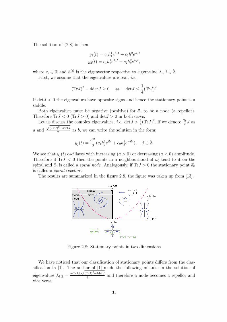
The results are summarized in the figure 2.8, the figure was taken up from [13].

Figure 2.8: Stationary points in two dimensions

We have noticed that our classification of stationary points differs from the clas-sification in [1]. The author of [1] made the following mistake in the solution of

eigenvalues λ1,2 =−TrJ±

√(TrJ)2−4detJ

2and therefore a node becomes a repellor and

vice versa.

31

Example 9. We try to find the character of stationary points of the following system

x = 3x− x2 − 2xy y = 2y − xy − y2.

This system has four stationary points: (0, 0), (0, 2), (1, 1) and (3, 0). We make upthe Jacobian matrix J and evaluate it in the stationary points to determine the typeof these stationary points.

J =

(

3 − 2x− 2y −2x−y 2 − x− 2y

)

(0, 0) J =

(

3 00 2

)

TrJ = 5 detJ = 6 ⇒ a repellor

(0, 2) J =

(

−1 0−2 −2

)

TrJ = −3 detJ = 2 ⇒ a node

(3, 0) J =

(

−3 −60 −1

)

TrJ = −4 detJ = 3 ⇒ a node

(1, 1) J =

(

−1 −2−1 −1

)

TrJ = −2 detJ = −1 ⇒ a saddle

♠

2.5.3 Three-dimensional case

We classify the stationary points in three-dimensional case quite quickly because itis practically the same as in the previous case. The dynamical system is describedby a system:

x1 = f1(x1, x2, x3)

x2 = f2(x1, x2, x3)

x3 = f3(x1, x2, x3).

The character of each stationary point x0 is fully determined by the eigenvaluesof the Jacobian matrix Jij = ∂fi

∂xj(x0). We do not try to find explicit form of each

eigenvalue as in the previous case because it is tremendous and for purposes ofinvestigating the stability also useless.

Definition 10. The number of eigenvalues of Jacobian matrix respective to sta-tionary point x0, whose real parts are positive, is called the index of the stationarypoint x0.

32

This term is introduced for systems with three or more dimension and in geometricterms, it is the dimension of the unstable subset Eu.

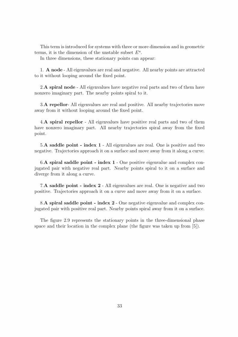
In three dimensions, these stationary points can appear:

1. A node - All eigenvalues are real and negative. All nearby points are attractedto it without looping around the fixed point.

2.A spiral node - All eigenvalues have negative real parts and two of them havenonzero imaginary part. The nearby points spiral to it.

3.A repellor- All eigenvalues are real and positive. All nearby trajectories moveaway from it without looping around the fixed point.

4.A spiral repellor - All eigenvalues have positive real parts and two of themhave nonzero imaginary part. All nearby trajectories spiral away from the fixedpoint.

5.A saddle point - index 1 - All eigenvalues are real. One is positive and twonegative. Trajectories approach it on a surface and move away from it along a curve.

6.A spiral saddle point - index 1 - One positive eigenvalue and complex con-jugated pair with negative real part. Nearby points spiral to it on a surface anddiverge from it along a curve.

7.A saddle point - index 2 - All eigenvalues are real. One is negative and twopositive. Trajectories approach it on a curve and move away from it on a surface.

8.A spiral saddle point - index 2 - One negative eigenvalue and complex con-jugated pair with positive real part. Nearby points spiral away from it on a surface.

The figure 2.9 represents the stationary points in the three-dimensional phasespace and their location in the complex plane (the figure was taken up from [5]).

33

Figure 2.9: Stationary points in three dimensions

34

Chapter 3

Chaotic oscillators

In this chapter, we would like to show that the chaotic behaviour is not the subjectlimited only to theoretical models but it occurs in real physical systems and thesesystems are often very simple.

We have chosen two electrical circuits and we try to analyze their behaviour.First, we look at the circuits analytically, and then we simulate their behaviourusing the ode15s MATLAB solver for stiff differential equations.

Before doing this, we briefly introduce the components of the circuit, their func-tion, and how they affect to the circuit behaviour.

A resistor - The current passing through a resistor is directly proportional tothe voltage across a resistor V = IR, where the proportionality constant R is calledthe resistance.

A capacitor - It is an electrical device that can store energy in the electricalfield V = Q

C. The measure C of the amount of charge Q stored in a capacitor is

called the capacitance.An inductor - The important property of an inductor is that it produces an

electrical potential difference across it: V = LdIdt

, where the proportionality constantL is called the inductance. It has to be emphasized that no chaotic circuit gets alongwithout an inductor. Without it, the current and potential differences are so tightlyjoined that there is no possibility for chaotic behaviour.

A diode - A diode is an electrical device, which allows an electrical currentto flow in one direction (this direction is called a forward-bias direction and it isindicated by the vertex of the triangle in diode´s circuit symbol), but blocks it inthe other (reverse-bias direction). We can understand the basic function of a diodeusing a hydraulic analogy. We imagine a diode as a water pipe with a flap valve.The valve can deflect in one direction to allow water to flow but it closes when watertries to flow in the opposite direction.

The first important property of the pipe with a flap valve (a diode) is that thevalve does not close immediately so a small amount of water (current) always passesthrough in the reverse-bias direction. The time necessary for closing is called thereverse-recovery time and it is usually a few microseconds.

The second property is that the reverse-recovery time depends on the flow volume

35

(the size of current). If only a small amount of water flows, the valve is deflectedjust a little bit and it can close quite fast. If we increase the flow volume, the valveneed more time for closing.

If we combine an inductor with a capacitor and if we put them in the circuit witha diode, while the frequency of circuit´s current oscillations (f = 2π√

LC) is about the

reverse-recovery time, the current is changing enough that the nonlinearity (changingthe forward-bias to reverse-bias current) becomes important and chaos becomespossible.

3.1 Vilnius oscillator

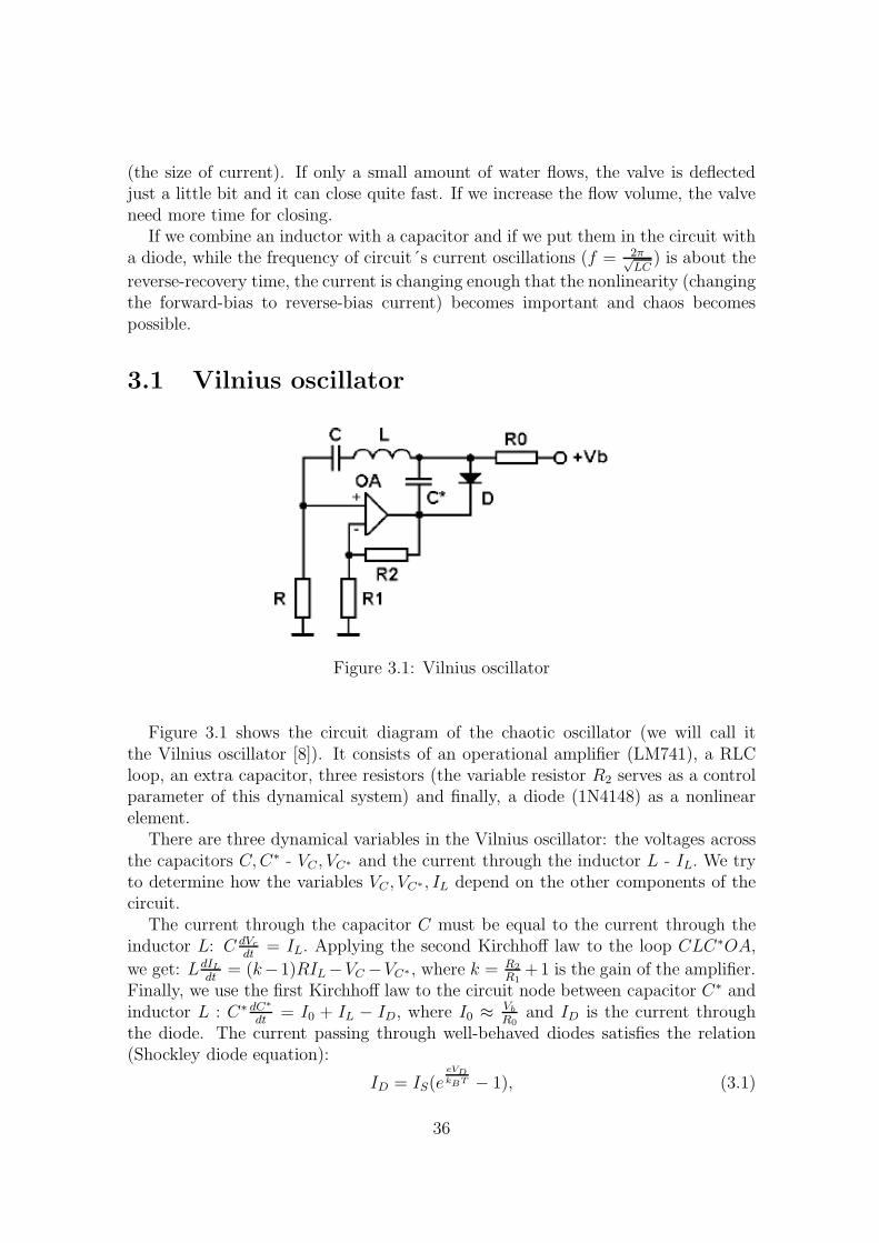
Figure 3.1: Vilnius oscillator

Figure 3.1 shows the circuit diagram of the chaotic oscillator (we will call itthe Vilnius oscillator [8]). It consists of an operational amplifier (LM741), a RLCloop, an extra capacitor, three resistors (the variable resistor R2 serves as a controlparameter of this dynamical system) and finally, a diode (1N4148) as a nonlinearelement.

There are three dynamical variables in the Vilnius oscillator: the voltages acrossthe capacitors C,C∗ - VC , VC∗ and the current through the inductor L - IL. We tryto determine how the variables VC , VC∗ , IL depend on the other components of thecircuit.

The current through the capacitor C must be equal to the current through theinductor L: C dVc

dt= IL. Applying the second Kirchhoff law to the loop CLC∗OA,

we get: LdIL

dt= (k−1)RIL−VC −VC∗ , where k = R2

R1

+1 is the gain of the amplifier.Finally, we use the first Kirchhoff law to the circuit node between capacitor C∗ andinductor L : C∗ dC∗

dt= I0 + IL − ID, where I0 ≈ Vb

R0

and ID is the current throughthe diode. The current passing through well-behaved diodes satisfies the relation(Shockley diode equation):

ID = IS(eeVDkBT − 1), (3.1)

36

where IS is the saturation current (characteristic of a diode), e is the elementarycharge, kB is the Boltzmann constant, T is the absolute temperature and VD is thevoltage across the diode. With regard to the parallel connection between the diodeand capacitor C∗, we obtain that VD = VC∗ .

Thus, we have a system of three differential equations describing the circuit be-haviour:

CdVc

dt= IL, L

dIl

dt= (k − 1)RIL − VC − VC∗ , C∗dC

∗

dt= I0 + IL − ID. (3.2)

We change the variables VC , VC∗ , IL (as well as the other characteristics of thecircuit components) for dimensionless ones, which are more convenient for numericalsimulations:

x =VC

VTy =

ρIL

VTz =

VC∗

VTθ =

t

τ

VT =kBT

eρ =

√

L

Cτ =

√LC a = (k − 1)

R

ρ(3.3)

b =ρI0

VT

c =ρIS

VT

ǫ =C∗

C.

The system (3.2) in new variables looks like:

x = y, y = −x+ ay − z, ǫz = b+ y − c(ez − 1), (3.4)

where the dot denotes the differentiation with respect to θ.In Semiconductor Physics Institute in Vilnius, the circuit was set up with the

following parameters: L = 100mH, C = 10nF, C∗ = 15nF, Vb = 20V, R = 1kΩ,R1 = 10kΩ, R0 = 20kΩ. The resistance of the variable resistor R2 ranges from 0to 10kΩ. The room temperature is fixed at the value T = 293, 15K. The saturationcurrent of a diode is IS = 1.10−13A (the value was derived from constant c used in anarticle [8]). We will use the same values of parameters for the numerical simulation.

Thus, a ∈ 〈0, 1〉, b = 39, 57, c = 4.10−9 and ǫ = 0.15.The system (3.4) has the only stationary solution (−ln(1 + b

c), 0, ln(1 + b

c)). We

determine how the nearby points behave and then we try to explain these resultsfrom a physical point of view.

We change the coordinates once more in order to arrange the stationary pointinto the origin:

u = x+ ln(

1 +b

c

)

v = y w = z − ln(

1 +b

c

)

. (3.5)

The system (3.4) transforms to the new system:

u = v, v = av − u− w, ǫw = b+ v − c(b+ c

cew − 1

)

. (3.6)

37

Unfortunately, we are unable to gain the eigenvalues of the linearized system

u = v, v = av − u− w, w =v

ǫ− b+ c

ǫw

in an analytical form. The stationary point is a saddle point - index 2, i.e. thelinearized system has two eigenvalues with positive real part and one with negativeone, as results from the numerical evaluations, which were done in the programMaple.

The instability of this fixed point is not surprising because it corresponds to thesituation when zero current passes through the inductor L although the current I0remains constant. This splitting of current (when the currents passing through C∗

and D are much more bigger than the inductor current) is very unsymmetric andthe circuit tries to return to the equilibrium.

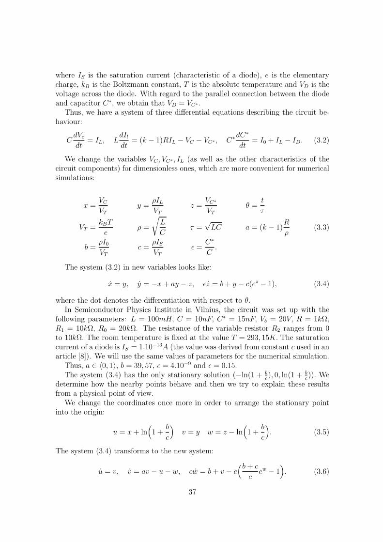
The solution of the system (3.4) with initial condition (−23, 0, 23) and a = 0.4 isillustrated in the figure 3.2.

−80 −60 −40 −20 0 20 40 60 80 100−100

−80

−60

−40

−20

0

20

40

60

80

100

x

y

Figure 3.2: Vilnius oscillator

3.2 Chaos generator

The nonlinear circuit, shown in the figure 3.3, is a simple RLC circuit. It consistsof two capacitors Cm, C, resistors Rm, R, an inductor L, an amplifier and a squaringmodule. The variable resistor Rm serves as a control parameter.

Applying the second Kirchhoff law to the loop RCCm, we get:

Q

C+R(Q+ Qm) − v2(U − U0)

2 = 0, (3.7)

where the dot denotes the differentiation with respect to time, Q and Qm are thecharges at C,Cm and U is the voltage at the capacitor Cm.

38

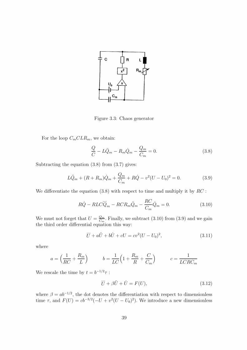
Figure 3.3: Chaos generator

For the loop CmCLRm, we obtain:

Q

C− LQm − RmQm − Qm

Cm

= 0. (3.8)

Subtracting the equation (3.8) from (3.7) gives:

LQm + (R +Rm)Qm +Qm

Cm+RQ− v2(U − U0)

2 = 0. (3.9)

We differentiate the equation (3.8) with respect to time and multiply it by RC :

RQ−RLC...Qm −RCRmQm − RC

CmQm = 0. (3.10)

We must not forget that U = Qm

Cm. Finally, we subtract (3.10) from (3.9) and we gain

the third order differential equation this way:

...U + aU + bU + cU = cv2(U − U0)

2, (3.11)

where

a =( 1

RC+Rm

L

)

b =1

LC

(

1 +Rm

R+

C

Cm

)

c =1

LCRCm

We rescale the time by t = b−1/2τ :

...U + βU + U = F (U), (3.12)

where β = ab−1/2, the dot denotes the differentiation with respect to dimensionlesstime τ, and F (U) = cb−3/2(−U + v2(U − U0)

2). We introduce a new dimensionless

39

variable x :

U = A−Bx

A =1

2v2(1 + 2v2U0 +

√

1 + 4v2U0) (3.13)

B = v−2√

1 + 4v2U0. (3.14)

The equation (3.12) in new variables looks as follows:

...x + βx+ x = f(x), (3.15)

where the nonlinear function f(x) = µx(1 − x) depends on a parameter µ =cb−3/2

√1 + 4v2U0.

Using the standard substitution, we rewrite the third order differential equationas a system of three first order differential equations:

x = y

y = z (3.16)

z = −βz − y + f(x).

The system (3.16) has two stationary points x1 = 0 and x2 = 1. They correspondto U1 = 1

2v2 (1 + 2v2U0 +√

1 + 4v2U0) and U2 = 12v2 (1 + 2v2U0 −

√1 + 4v2U0). We

use the Hurwitz´s criterion for determining their stability.First, we create the Jacobian matrix of the system (3.16).

J =

0 1 00 0 1

µ− 2µx −1 −β

For x1 = 0, we obtain this characteristic equation of the Jacobian matrix J :

λ3 + βλ2 + λ− µ = 0. (3.17)

We see that the equation (3.17) does not satisfy even the necessary condition forstability. Therefore it is an unstable stationary point.

For x2 = 1, we obtain this characteristic equation of the Jacobian matrix J :

λ3 + βλ2 + λ+ µ = 0. (3.18)

All coefficients are positive, so we can set up the Hurwitz´s matrix respective to theequation (3.18):

1 µ 01 β 10 0 1

.

D1 = 1 > 0 D2 = β − µ D3 = D2

40

The stationary point x2 = 1 (U2 = 12v2 (1 + 2v2U0 −

√1 + 4v2U0) is stable for β > µ.

The behaviour in the neighbourhood of this stationary point will be studied in amore detail using the numerical simulation.

For β > µ, the stationary point is stable, for β < µ, it becomes unstable. Fromthe previous, it is obvious that a bifurcation occurs for β = µ. β and µ are bothfunctions of Rm so we expect that the bifurcation occurs when Rm increases ordecreases its critical value.

The values of circuit components used for the numerical simulations are the fol-lowing:

v = 1, 2V −1/2 R = 3300Ω C = Cm = 47.10−9F L = 0.1H U0 = 4V.

The stability condition β > µ tends to quadratic equation for Rm with only onepositive root. Hence for large values of Rm the voltage U remains at U2 = 2, 6447V .When Rm decreases its critical value Rmcrit = 770, 6113Ω, a Hopf bifurcation occurs,i.e. the limit cycle appears. For even smaller values of Rm, the system becomeschaotic.

The fact that just Hopf bifurcation ocurs results from characteristic equation(3.18). For β = µ, there is one real eigenvalue λ = −β and a complex conjugatedpair λ1,2 = ±i. From (3.18), it is also obvious that none of bifurcation, when a singlereal eigenvalue crosses the imaginary axis, can occur because of positivity of µ.

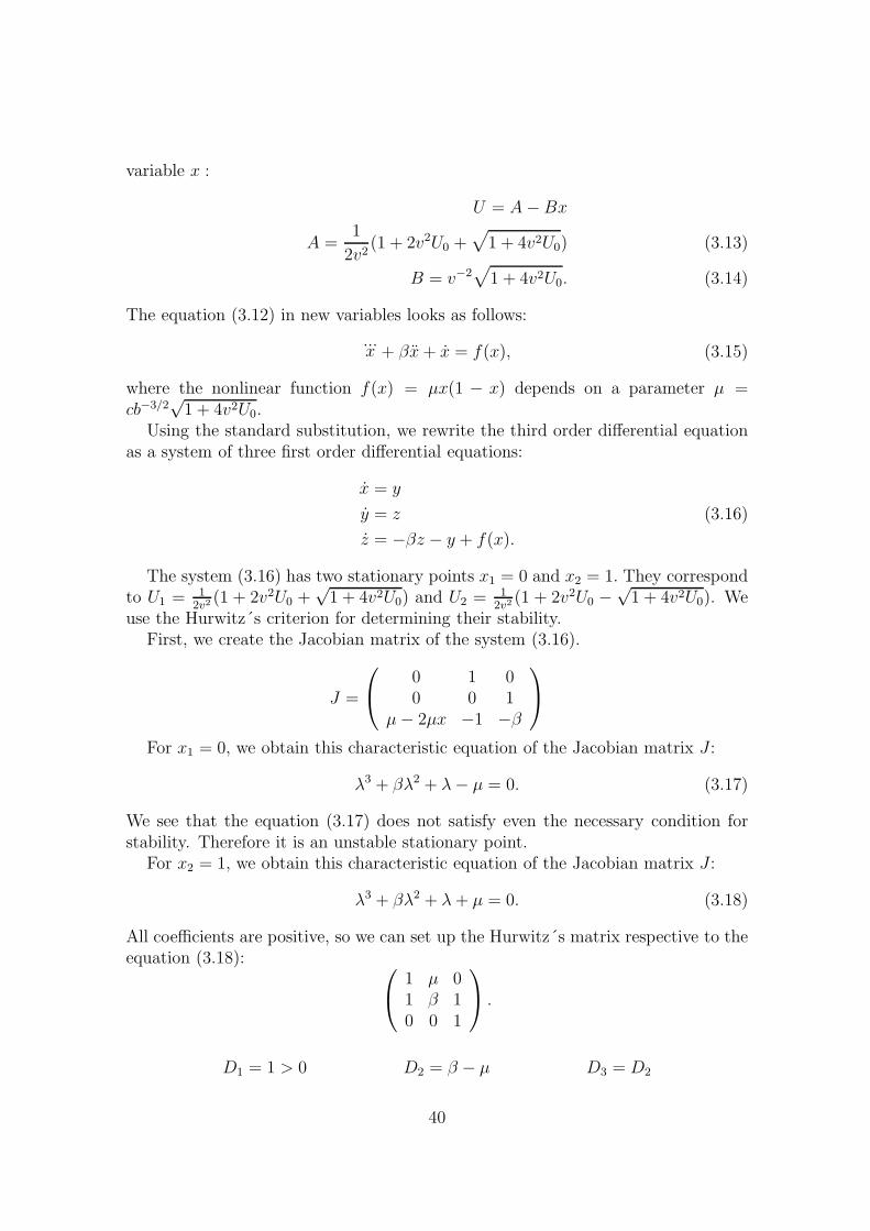
For Rm = 1000Ω, the system is damped down and all points from a neighbour-hood of the stationary point x2 tend to it. This situation is illustrated in the figure3.4 for the initial condition (1, 78; 0; 0). The stationary point attraction is shown inthe left figure and the signal damping in the right one.

0.2 0.4 0.6 0.8 1 1.2 1.4 1.6 1.8−0.8

−0.6

−0.4

−0.2

0

0.2

0.4

0.6

x

y

0 20 40 60 80 1000.2

0.4

0.6

0.8

1

1.2

1.4

1.6

1.8

t

x

Figure 3.4: Stable stationary point

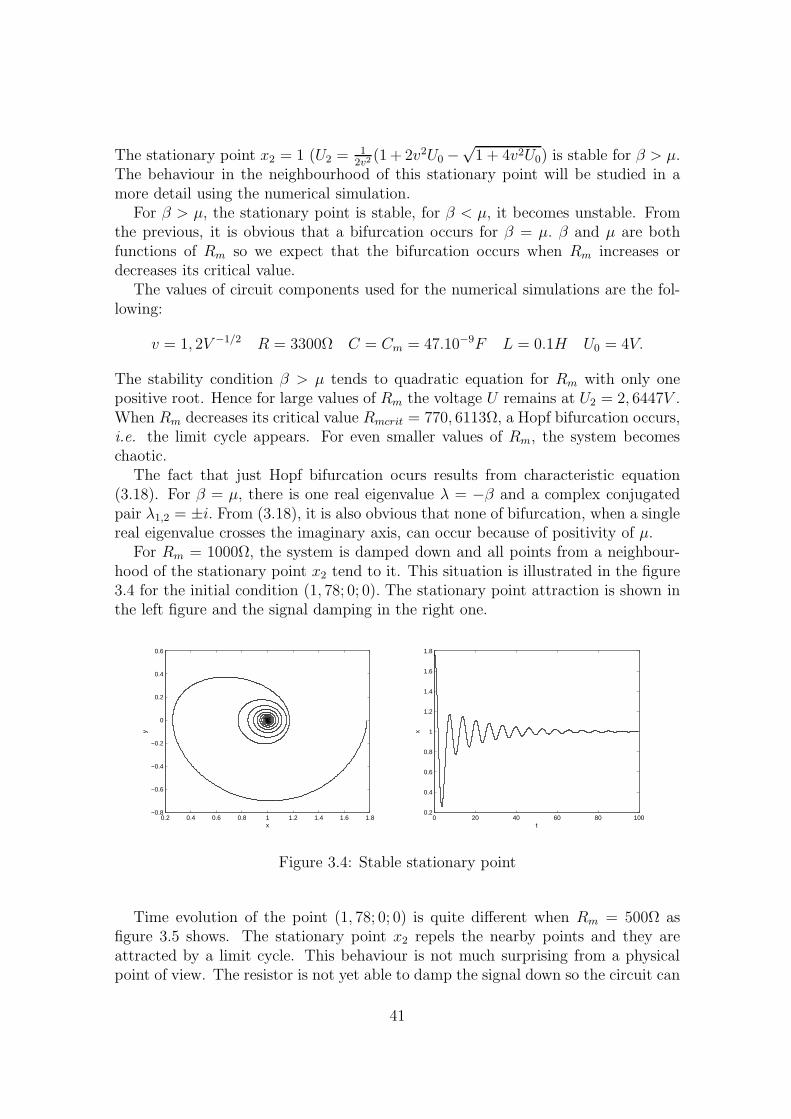
Time evolution of the point (1, 78; 0; 0) is quite different when Rm = 500Ω asfigure 3.5 shows. The stationary point x2 repels the nearby points and they areattracted by a limit cycle. This behaviour is not much surprising from a physicalpoint of view. The resistor is not yet able to damp the signal down so the circuit can

41

begin to oscillate. The variables U, U (scaled x, y) oscillate with the same frequencyso the phase trajectory is an ellipse.

0 0.2 0.4 0.6 0.8 1 1.2 1.4 1.6 1.8−1

−0.5

0

0.5

x

y

0 20 40 60 80 1000

0.2

0.4

0.6

0.8

1

1.2

1.4

1.6

1.8

t

x

Figure 3.5: Limit cycle

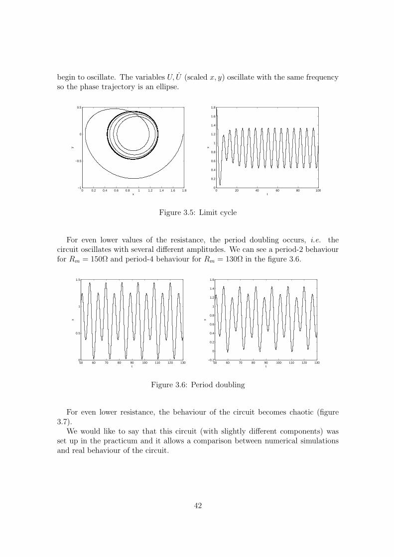
For even lower values of the resistance, the period doubling occurs, i.e. thecircuit oscillates with several different amplitudes. We can see a period-2 behaviourfor Rm = 150Ω and period-4 behaviour for Rm = 130Ω in the figure 3.6.

50 60 70 80 90 100 110 120 1300

0.5

1

1.5

t

x

50 60 70 80 90 100 110 120 130−0.2

0

0.2

0.4

0.6

0.8

1

1.2

1.4

1.6

t

x

Figure 3.6: Period doubling

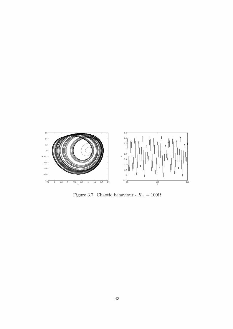
For even lower resistance, the behaviour of the circuit becomes chaotic (figure3.7).

We would like to say that this circuit (with slightly different components) wasset up in the practicum and it allows a comparison between numerical simulationsand real behaviour of the circuit.

42

−0.2 0 0.2 0.4 0.6 0.8 1 1.2 1.4 1.6−1

−0.8

−0.6

−0.4

−0.2

0

0.2

0.4

0.6

x

y

50 100 150−0.2

0

0.2

0.4

0.6

0.8

1

1.2

1.4

1.6

t

x

Figure 3.7: Chaotic behaviour - Rm = 100Ω

43

Bibliography

[1] P. Glendinning, Stability, instability and chaos: an introduction to the theory of

nonlinear differential equations, Cambridge University Press, Cambridge, 1996

[2] J. Kofron, Obycejne diferencialnı rovnice v realnem oboru, NakladatelstvıKarolinum, Praha, 2004

[3] P.G.Drazin, Nonlinear systems, Cambridge Univerisity Press, Cambridge, 1994

[4] J. D. Crawford , Introduction to bifurcation theory, Review of Modern Physics,Vol.63, No.4,October 1991

[5] R. C. Hilborn, Chaos and nonlinear dynamics: An introduction for scientists

and engineers, Oxford Univerisity Press, Oxford, 2004

[6] J. Fiala, a L. Skala, Uvod do nelinearnı fyziky, Matfyzpress, Praha, 2003

[7] B. P. Demidovic, Lekcii po mateticeskoj teorii ustojcivosti, Nauka, Moskva,1967

[8] A.Tamasevicius, G.Mykolaitis, V.Pyragas, and K.Pyragas, A simple chaotic

oscillator for educational puproses, European Journal of Physics 26, 2005

[9] P. K. Roy, and A. Basuray, A high frequency chaotic signal generator: A demon-

stration experiment, American Journal of Physics 71(1), January 2003

[10] P. Horowitz, and W. Hill, The art of electronics, Cambridge University Press,Cambridge, 1989

[11] H.J.Korsch, and H.J.Jodl, Chaos: A program collecting for the PC, Springer -Verlag, Berlin, 1994

[12] R.Cerna, S.Cipera, a F.Peterka, Numericke simulace dynamickych systemu, Vy-davatelstvı CVUT, Praha, 1995

[13] http://monet.physik.unibas.ch/∼elmer/pendulum/bif.htm

44

ProhlasenıProhlasuji, ze jsem svou bakalarskou praci vypracovala samostatne a pouzila jsem

pouze podklady uvedene v prilozenem seznamu.Nemam zadny duvod proti uzitı tohoto skolnıho dıla ve smyslu §60 Zakona c.

121/2000 Sb., o pravu autorskem, o pravech souvisejıcıch s pravem autorskym a ozmene nekterych zakonu (autorsky zakon).

DeclarationI declare that I wrote my bachelor thesis independently and exclusively with the

use of cited bibliography.I agree with the usage of this thesis in a purport of the Act 121/2000 (Copyright

Act).

Praha, July 21, 2007

Lucie Strmiskova

45