CRISTIAN QUISPE VENTURA

CÓDIGO: 12190027

CURSO: LABORATORIO DE SISTEMAS DE CONTROL 1

TEMA: TRANSFORMADA DE LAPLACE Y FRACIONES PARCIALES INFORME 3

PROFESOR: HILDA

DESARROLLO DEL CUESTIONARIO:

OBTENER LA TRANSFORMADA DE LAPLACE, SUS GRÁFICOS RESPECTIVOS DE LAS SIGUIENTES FUNCIONES TEMPORALES.

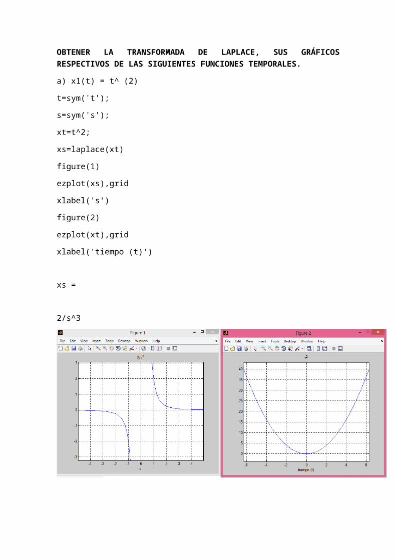
a) x1(t) = t^ (2)

t=sym('t');

s=sym('s');

xt=t^2;

xs=laplace(xt)

figure(1)

ezplot(xs),grid

xlabel('s')

figure(2)

ezplot(xt),grid

xlabel('tiempo (t)')

xs =

2/s^3

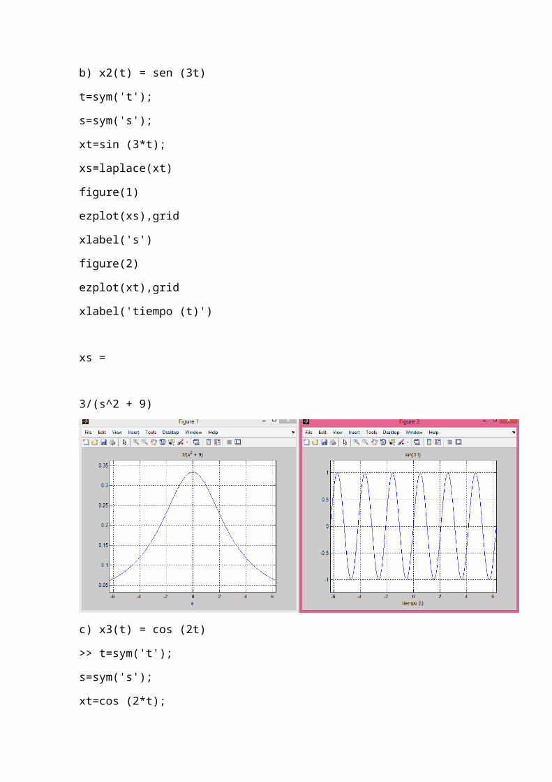
b) x2(t) = sen (3t)

t=sym('t');

s=sym('s');

xt=sin (3*t);

xs=laplace(xt)

figure(1)

ezplot(xs),grid

xlabel('s')

figure(2)

ezplot(xt),grid

xlabel('tiempo (t)')

xs =

3/(s^2 + 9)

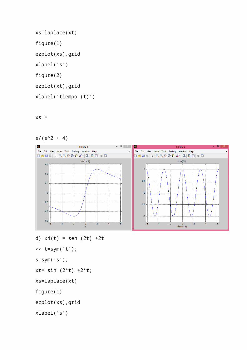
c) x3(t) = cos (2t)

>> t=sym('t');

s=sym('s');

xt=cos (2*t);

xs=laplace(xt)

figure(1)

ezplot(xs),grid

xlabel('s')

figure(2)

ezplot(xt),grid

xlabel('tiempo (t)')

xs =

s/(s^2 + 4)

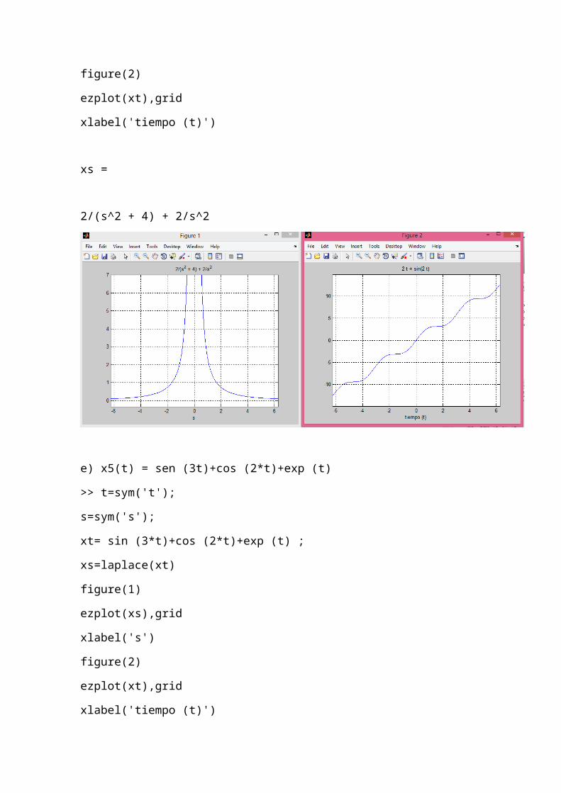
d) x4(t) = sen (2t) +2t

>> t=sym('t');

s=sym('s');

xt= sin (2*t) +2*t;

xs=laplace(xt)

figure(1)

ezplot(xs),grid

xlabel('s')

figure(2)

ezplot(xt),grid

xlabel('tiempo (t)')

xs =

2/(s^2 + 4) + 2/s^2

e) x5(t) = sen (3t)+cos (2*t)+exp (t)

>> t=sym('t');

s=sym('s');

xt= sin (3*t)+cos (2*t)+exp (t) ;

xs=laplace(xt)

figure(1)

ezplot(xs),grid

xlabel('s')

figure(2)

ezplot(xt),grid

xlabel('tiempo (t)')

xs =

1/(s - 1) + s/(s^2 + 4) + 3/(s^2 + 9)

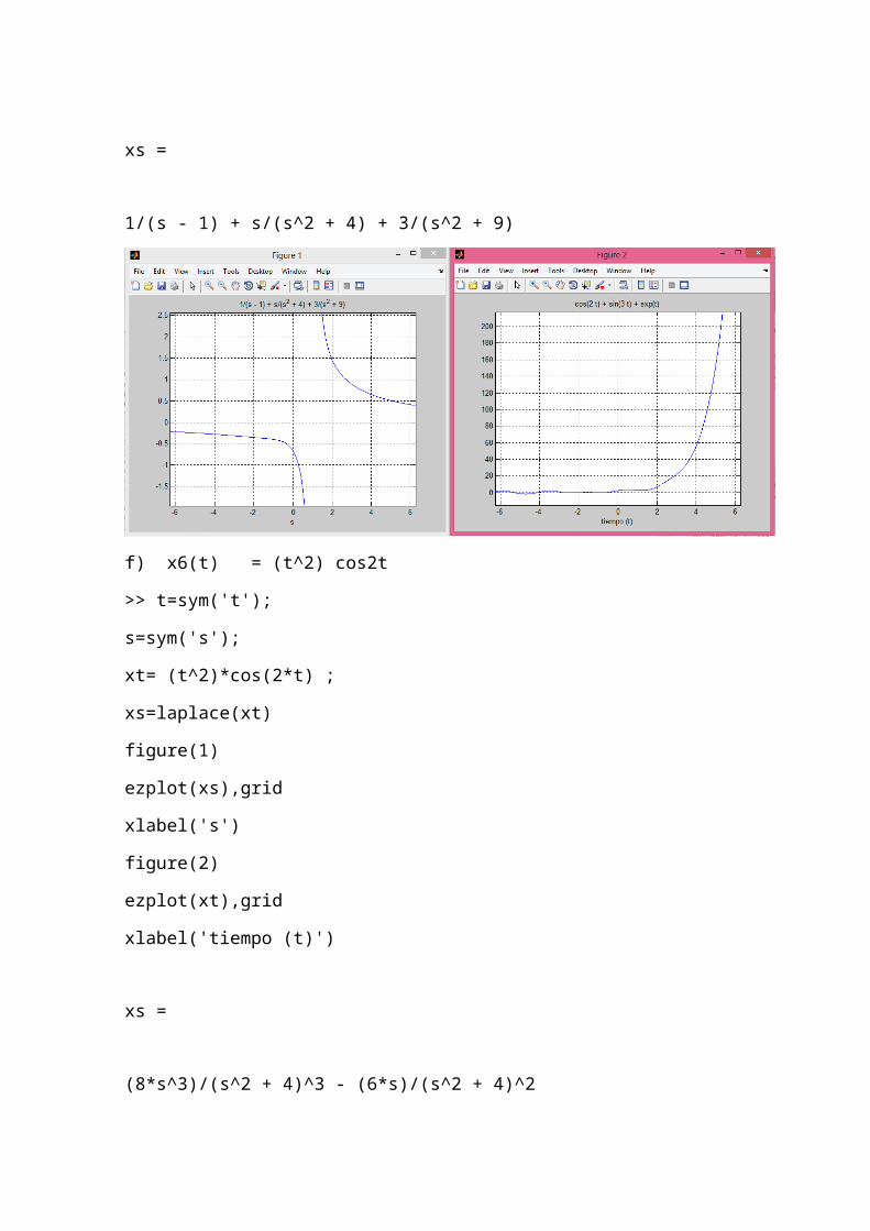
f) x6(t) = (t^2) cos2t

>> t=sym('t');

s=sym('s');

xt= (t^2)*cos(2*t) ;

xs=laplace(xt)

figure(1)

ezplot(xs),grid

xlabel('s')

figure(2)

ezplot(xt),grid

xlabel('tiempo (t)')

xs =

(8*s^3)/(s^2 + 4)^3 - (6*s)/(s^2 + 4)^2

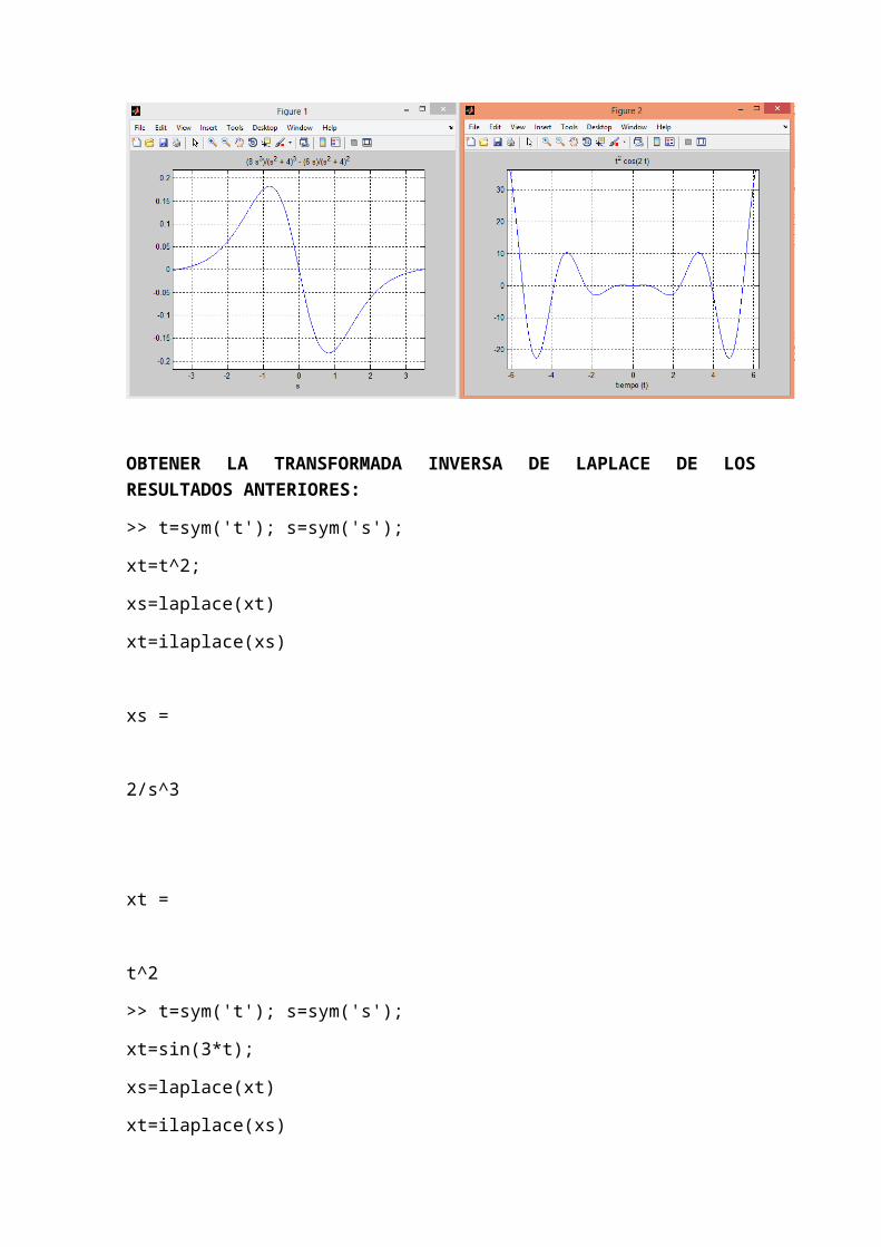
OBTENER LA TRANSFORMADA INVERSA DE LAPLACE DE LOS RESULTADOS ANTERIORES:

>> t=sym('t'); s=sym('s');

xt=t^2;

xs=laplace(xt)

xt=ilaplace(xs)

xs =

2/s^3

xt =

t^2

>> t=sym('t'); s=sym('s');

xt=sin(3*t);

xs=laplace(xt)

xt=ilaplace(xs)

xs =

3/(s^2 + 9)

xt =

sin(3*t)

>> t=sym('t'); s=sym('s');

xt=cos(2*t);

xs=laplace(xt)

xt=ilaplace(xs)

xs =

s/(s^2 + 4)

xt =

cos(2*t)

>> t=sym('t'); s=sym('s');

xt=sin(2*t)+2*t;

xs=laplace(xt)

xt=ilaplace(xs)

xs =

2/(s^2 + 4) + 2/s^2

xt =

2*t + sin(2*t)

>> t=sym('t'); s=sym('s');

xt=sin(3*t)+cos(2*t)+exp(t) ;

xs=laplace(xt)

xt=ilaplace(xs)

xs =

1/(s - 1) + s/(s^2 + 4) + 3/(s^2 + 9)

xt =

cos(2*t) + sin(3*t) + exp(t)

>> t=sym('t');

s=sym('s');

xt= (t^2)*cos(2*t) ;

xt=ilaplace(xs)

xt =

t^2*cos(2*t)

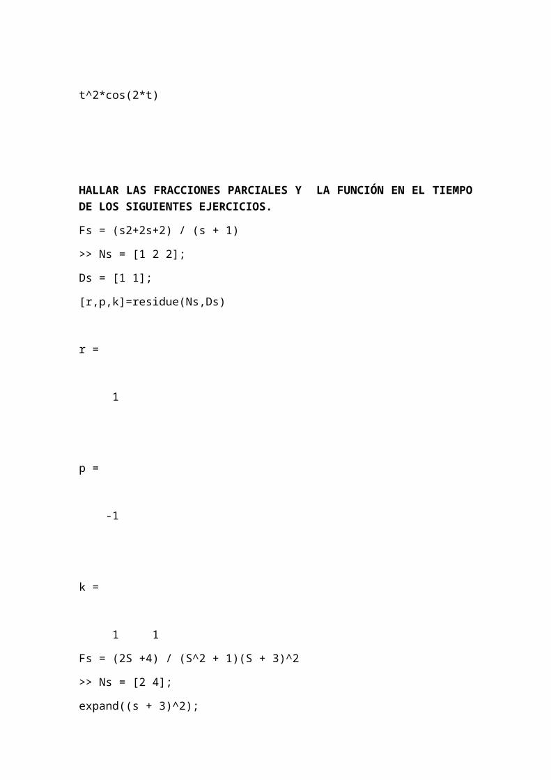
HALLAR LAS FRACCIONES PARCIALES Y LA FUNCIÓN EN EL TIEMPO DE LOS SIGUIENTES EJERCICIOS.

Fs = (s2+2s+2) / (s + 1)

>> Ns = [1 2 2];

Ds = [1 1];

[r,p,k]=residue(Ns,Ds)

r =

1

p =

-1

k =

1 1

Fs = (2S +4) / (S^2 + 1)(S + 3)^2

>> Ns = [2 4];

expand((s + 3)^2);

d1 = [1 0 1];

d2 = [1 6 9];

Ds=conv(d1,d2);

[r,p,k]=residue(Ns,Ds)

r =

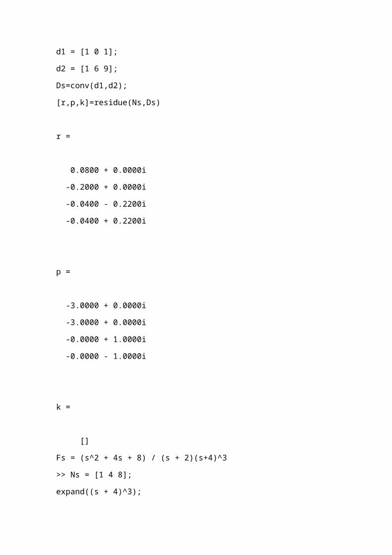
0.0800 + 0.0000i

-0.2000 + 0.0000i

-0.0400 - 0.2200i

-0.0400 + 0.2200i

p =

-3.0000 + 0.0000i

-3.0000 + 0.0000i

-0.0000 + 1.0000i

-0.0000 - 1.0000i

k =

[]

Fs = (s^2 + 4s + 8) / (s + 2)(s+4)^3

>> Ns = [1 4 8];

expand((s + 4)^3);

d1 = [1 2];

d2 = [1 12 48 64];

Ds=conv(d1,d2);

[r,p,k]=residue(Ns,Ds)

r =

-0.5000

-0.0000

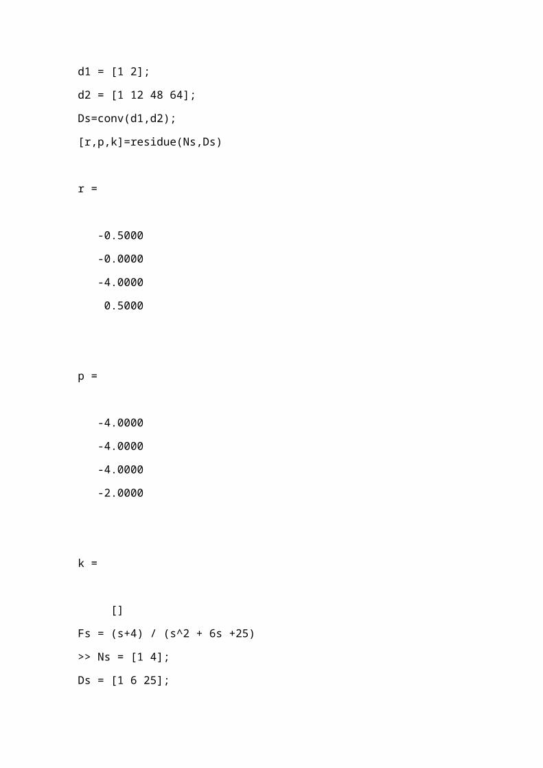
-4.0000

0.5000

p =

-4.0000

-4.0000

-4.0000

-2.0000

k =

[]

Fs = (s+4) / (s^2 + 6s +25)

>> Ns = [1 4];

Ds = [1 6 25];

[r,p,k]=residue(Ns,Ds)

r =

0.5000 - 0.1250i

0.5000 + 0.1250i

p =

-3.0000 + 4.0000i

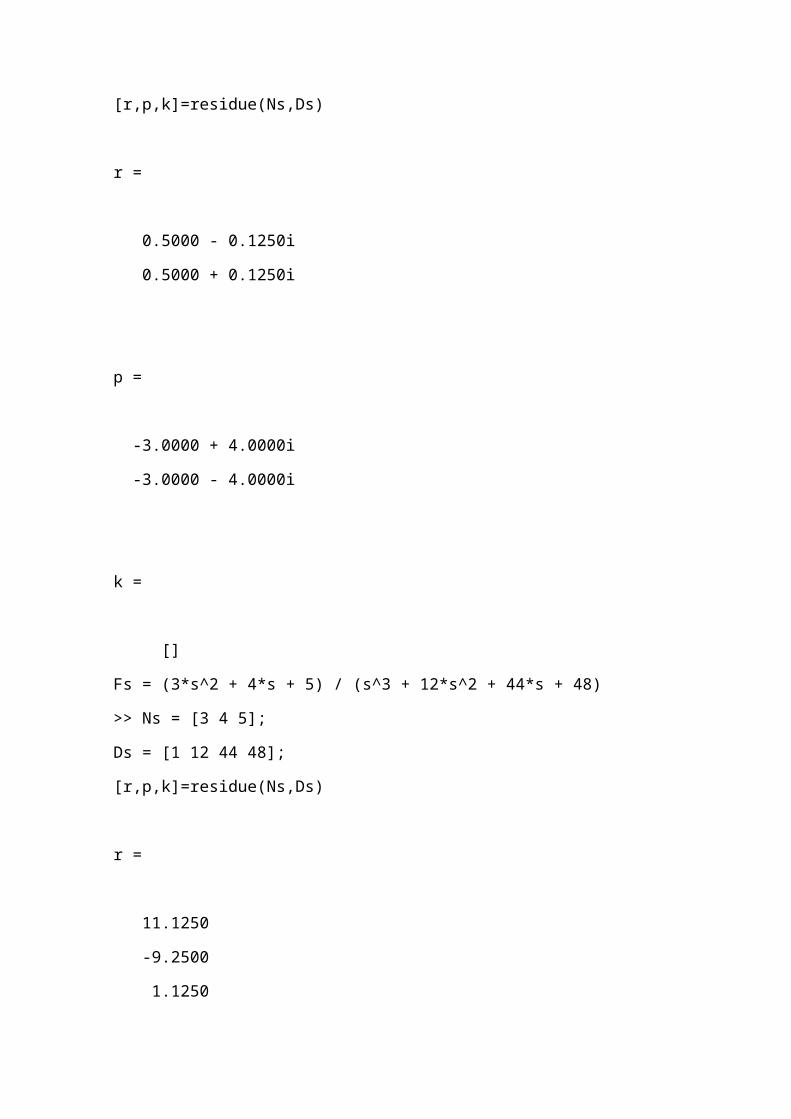
-3.0000 - 4.0000i

k =

[]

Fs = (3*s^2 + 4*s + 5) / (s^3 + 12*s^2 + 44*s + 48)

>> Ns = [3 4 5];

Ds = [1 12 44 48];

[r,p,k]=residue(Ns,Ds)

r =

11.1250

-9.2500

1.1250

p =

-6.0000

-4.0000

-2.0000

k =

[]